Read the public excerpt
The same instruction and worked examples appear here and in the printable PDF excerpt. You can request full guides for upcoming units below.
READ THIS FIRST
About this guide. Unit 2 is where the course stops describing data it has and starts reasoning about data it does not have yet. Every tool in it — a two-way table, a simulation, a probability rule, a random variable, the binomial and normal distributions, a sampling distribution — is a way of saying how often something would happen over the long run, and the whole of Units 3 through 5 stands on that. A confidence interval is a normal calculation from this unit; a -value is a sampling-distribution probability from this unit; a chi-square test is a two-way table from this unit. Learn this one properly and the rest of the course is one idea applied four times.
The College Board’s own note on the unit is about showing the structure: a probability calculation on the exam “needs to include presentation of an appropriate expression that communicates the structure of the formula, substitution of relevant values extracted from the problem, and an answer,” and a distribution calculation is expected to include “identifying the distribution, labeling relevant values extracted from the problem, and indicating boundaries and direction.” That sentence is the rubric, and every worked problem below writes to it.
Three mistakes to learn to catch:
- A probability with no structure behind it. alone earns the answer’s point and none of the method’s; earns them all. The calculator’s number is the last line, never the only one.
- “Mutually exclusive” and “independent” used as synonyms. They are close to opposites: two events that cannot happen together are as dependent as events get, because one happening tells you the other did not. The unit’s most-missed multiple-choice question lives on that distinction.
- A parameter described instead of interpreted. “The mean is 1.75” describes the table; “over many plays, a player wins an average of $1.75 per play” interprets it. The CED says students “simply describe features of the graph rather than explicitly connecting those features to the situation,” and the point is in the connecting.
Every topic in the unit, and where it lives. The College Board lists twelve; here is each one and the page that teaches it.
- 2.1, 2.2 two categorical variables: the two-way table, joint, marginal and conditional relative frequencies, association — card 2 (p. 12); Problem 1.
- 2.3 probability as long-run relative frequency, and simulation — card 3 (p. 13); Problem 2.
- 2.4, 2.5 sample spaces, complements, mutually exclusive events — card 4 (p. 15); Problem 3.
- 2.6, 2.7 conditional probability, the multiplication rule, independence, unions — cards 4 and 5 (p. 17); Problems 3 and 4.
- 2.8, 2.9 discrete random variables, their distributions, their mean and standard deviation — card 6 (p. 18); Problem 5.
- 2.10 the binomial distribution — card 7 (p. 20); Problem 6.
- 2.11 the normal distribution — card 8 (p. 22); Problem 7.
- 2.12 sampling distributions, randomization distributions, the central limit theorem — card 9 (p. 24); Problem 8.
How to use it. The decision tree, the symptom map and the Master Toolbox are reference, not assigned reading. Route the problem, open the matching card, and attempt the prompt before reading the worked solution. The exam allows a graphing calculator with statistical capabilities in both sections and supplies a formula sheet and tables; what it does not supply is the sentence that names the distribution and the boundary, which is where the points are. What eight problems cannot do is give you enough repetitions; each is the clearest instance of its shape, so a problem you found easy is a signal to go find five more like it.
WHERE THE POINTS GO ON THIS UNIT
On the exam as it stood in 2025, six free-response questions worth 24 points, the average student earned 42.8% of them; the revised exam’s published rubric for one ten-point inference question puts one point on the calculation and nine on the sentences around it. In this unit the sentences have names.
Each of those sentences is a separate job: write the event, name the model and its parameters, show the boundary you used, then say what the number means for the people or the process in front of you. A calculator output does exactly one of the four.
The structure, the substitution, the answer. The CED’s own words: a calculation “needs to include presentation of an appropriate expression that communicates the structure of the formula, substitution of relevant values extracted from the problem, and an answer.” Three lines, every time — , then , then . A student who writes only the third has given the grader nothing to award the method for.
Name the distribution, label the values, show the boundary and the direction. For a binomial or normal calculation the rubric wants “identifying the distribution, labeling relevant values extracted from the problem, and indicating boundaries and direction”: , ; or , , with the curve sketched, shaded and labeled. A calculator command alone — binomcdf(12,0.7,9) — is not a distribution named.
Context and units on every parameter. Students “frequently misinterpret probability distributions and parameters for random variables”; a complete interpretation “includes context and units.” The mean of a random variable is a long-run average of something, in some unit, per something; the standard deviation is a typical distance from that average in the same unit.
Not every probability is a test. The CED flags “a common misconception later in the course …that every question involving probability requires a significance test.” A question that asks how likely a sample mean above 225 minutes is, is answered with a sampling-distribution probability and a sentence — no hypotheses, no . Learn here what a probability question looks like, so Unit 4 does not turn every one into a procedure.
Independent is not mutually exclusive. Check independence with numbers — against , or against — and say which check you ran. Mutually exclusive means . Two events with positive probability cannot be both.
Diagnostic Decision Tree
WHAT IS BEING ASKED, AND WHAT KIND OF OBJECT ANSWERS IT
Run these in order, before touching a formula or a calculator. Each one rules out whole families of tools.
1. Data you have, or a chance you are asked about? Two categorical variables in a table with counts — describe and compare with relative frequencies, and the question is association. A question about how likely something is — everything below.
2. Can it be simulated, or must it be computed? “Describe a process using random digits” wants a simulation: assign digits to outcomes, say what one trial is, say what is recorded, say how many trials, and estimate by relative frequency. A theoretical probability wants a rule.
3. Which word is in the question? Or — the addition rule, minus the overlap. And — the multiplication rule, with the conditional. Given — a conditional: the intersection over the condition. At least one — the complement of none. Neither — the complement of the union. Card 5 is the picker.
4. Is a random variable named? A count or a measurement with probabilities attached is a random variable; its distribution is a table that sums to 1, and its mean and standard deviation are computed from the table and interpreted in context, with units.
5. Is it a count of successes in a fixed number of independent trials? Binary outcome, independent trials, fixed , the same — binomial. Name it, , write the boundary as an inequality, and let the calculator do the sum. If a condition fails — no fixed , draws without replacement from a small population — it is not binomial, and saying which condition fails is the answer.
6. Is it a continuous measurement with a stated normal model? Sketch, shade, label the mean and the boundary in original units, standardize, and read the area. Without the model stated or justified, the area is not licensed.
7. Is the question about a statistic — a sample mean or proportion — rather than one individual? Then the object is a sampling distribution, and three things get said before anything is computed: its center is the parameter, its standard deviation is the population’s divided by , and its shape is approximately normal by the central limit theorem when is large enough or the population is normal. Card 9 carries the conditions each of those three rests on. And a large buys the shape, not the sample: it does not repair biased sampling.
Where to Look When You’re Stuck
FIND THE SENTENCE THAT SOUNDS LIKE YOUR SITUATION
What is happening | First move | Where |
|---|---|---|
“Which total do I divide by?” | Joint: the grand total. Marginal: the grand total. Conditional: the total of the row or column you were given. | p. 12, Prob. 1 |
“Is there an association or not?” | Compare conditional distributions across the levels of the other variable; different means associated. | p. 12, Prob. 1 |
“It says describe a simulation” | Digits to outcomes, one trial, what is recorded, how many trials, the estimate as a relative frequency. | p. 13, Prob. 2 |
“Or, and, given — which formula?” | The word picks the rule; the picker card has all five. | p. 17, Prob. 3 |
“Are they independent?” | Compute and compare it with ; say which check you ran. Never decide from the words alone. | p. 15, Prob. 3 |
“The probability runs backwards — given the test, what is the disease?” | A tree, then Bayes by hand: the intersection over the total probability of the condition. | p. 17, Prob. 4 |
“I have a table of values and probabilities” | A random variable. Check it sums to 1, then and . | p. 18, Prob. 5 |
“Is it binomial?” | Binary, independent, fixed , same . All four or it is not. | p. 20, Prob. 6 |
“At least, at most, more than” | Write the inequality in first, then decide which calculator function covers it. | p. 20, Prob. 6 |
“A normal probability” | Sketch, shade, label; standardize; the area. State the model. | p. 22, Prob. 7 |
“It is asking about a sample mean, not a person” | Sampling distribution: center , spread , shape by the CLT. | p. 24, Prob. 8 |
“I have a number and no sentence” | Context and units: what is this a probability of, for whom, over what run? | Stuck Toolkit |
Master Toolbox — Everything These Problems Use
Use these cards as you work. Name the decision you need to make, then open the relevant card. Each card stands on its own; you do not need to read the whole toolbox before attempting a problem.
1. THE TASK VERB, AND THE THREE LINES EVERY CALCULATION SHOWS
Calculate | the expression with the structure of the formula, the substitution of the values from the problem, the answer — three lines, and the first two are where the method points live. |
|---|---|
Estimate (simulation) | a described process, the recorded statistic, the number of trials, and the estimate as a relative frequency. |
Interpret | the number, in context, with units, as a long-run statement: what it is a probability or an average of , for whom. |
Justify | the check and its numbers: , so not independent. The words alone are a guess. |
Describe / construct | the distribution’s name and parameters, or the table that sums to 1, or the sketch shaded and labeled. |
2. TWO CATEGORICAL VARIABLES: THE TWO-WAY TABLE AND THE THREE RELATIVE FREQUENCIES
A two-way table (contingency table) counts observational units by two categorical variables at once. Everything in Topics 2.1 and 2.2 is one question — which total do I divide by? — asked three ways:
- joint relative frequency: a cell over the grand total — the share of everyone who is both things;
- marginal relative frequency: a row or column total over the grand total — the share of everyone who is one thing, ignoring the other variable;
- conditional relative frequency: a cell over its row total or its column total — the share among the people in that row or column.
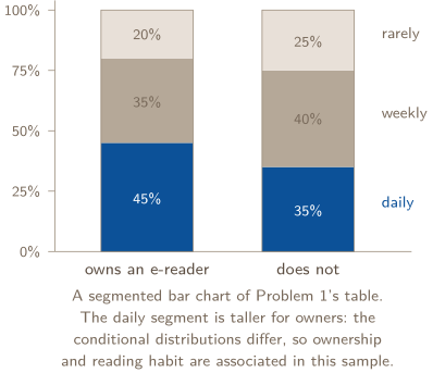
The conditional is the one that answers questions about association: if the conditional distribution of one variable differs across the levels of the other — 45% of device owners read daily against 35% of non-owners — the variables are associated. If the conditional distributions are the same at every level, they are not. Association is a claim about the sample; whether it travels to the population is Unit 5’s chi-square question.
The displays. A side-by-side bar chart puts the conditional distributions next to each other; a segmented bar chart stacks each conditional distribution to 100%, so association reads as segments of different heights; a mosaic plot is a segmented bar chart whose bar widths are the marginal proportions.
3. PROBABILITY IS A LONG-RUN RELATIVE FREQUENCY — AND A SIMULATION IS HOW YOU WATCH IT
A random process produces results determined by chance; one run of it is a trial, the result of a trial is an outcome, and a collection of outcomes is an event. The probability of an event is its long-run relative frequency — the fraction of trials in which it occurs, as the number of trials grows without bound. That is a definition, not a metaphor, and the law of large numbers is the theorem behind it: for independent trials, the relative frequency settles closer and closer to one value.
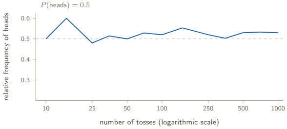
This is one simulated sequence, shown at selected checkpoints: 5 heads in the first 10 tosses and 530 in the first 1,000. Equal horizontal steps represent equal multiplicative changes in the toss count. A larger number of trials usually makes the relative frequency more stable; it need not move closer to at every step. A run of tails does not make heads “due”: each independent toss still has probability of heads.
A simulation, described so a grader can run it. Five parts, and the exam scores each:
- 1.
- assign digits (or cards, or a spinner) to outcomes so the probabilities match — “let 0–4 represent a girl and 5–9 a boy”;
- 2.
- one trial: what is read and how much — “read three digits; that is one family of three”;
- 3.
- record: the statistic from the trial — “count the girls; note whether the count is at least 2”;
- 4.
- repeat: many trials — “repeat for 20 families,” and on the exam “many times” means a stated large number;
- 5.
- estimate: the relative frequency — “the proportion of the 20 families with at least two girls estimates the probability.”
A simulation estimates; more independent trials reduce the typical sampling error, although an individual estimate can move farther away before moving closer. Problem 2 runs one against a digit table and compares it with the exact answer.
A check first. One question opens each of the next three cards and is answered where that card ends. Answer it before you read on; getting it wrong is the point, because that is what makes the card stick.
1. CHOOSE THE DENOMINATOR
Of 1,000 people screened, 10 have the condition. Nine of those ten test positive, and 99 of the people without it test positive as well. Of everyone who tests positive, what fraction actually has the condition?
4. THE RULES OF PROBABILITY — AND THE PICTURE THAT MAKES THEM OBVIOUS
The sample space is the set of all possible non-overlapping outcomes; its probability is . When the outcomes are equally likely,
and every probability is a number in . The complement of — written , or , “not ” — has , which is the fastest route to every “at least one” question in the course.
Two events at once. The joint probability is the chance both occur. Events are mutually exclusive (disjoint) when they cannot occur together: . The conditional probability of given is
the share of ’s probability in which also happens — and it is read straight off a two-way table as a cell over its row or column total. Rearranged, it is the general multiplication rule:
Independence: and are independent when knowing one happened does not change the probability of the other — , equivalently , equivalently . Any one of the three, checked with numbers, is the justification; the third is the multiplication rule for the independent case. And the addition rule for the union, “ or or both”:
the overlap subtracted once because adding and counted it twice. For mutually exclusive events the overlap is and the rule is a plain sum.
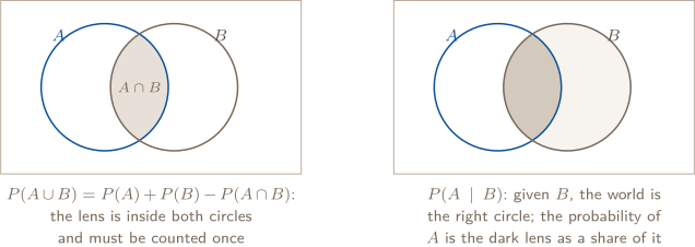
The distinction the exam tests most. Mutually exclusive is a statement about overlap (none); independent is a statement about information (none). Two events with positive probability that are mutually exclusive are dependent: if happened, certainly did not, so . Do not let the words decide either one — compute.
CHECK 1 — CHOOSE THE DENOMINATOR
, about one in twelve. The word given — here hidden inside “of everyone who tests positive” — names the denominator, and the denominator is every positive test: the true ones plus the false ones. Dividing by instead answers a different question (of those who have it, what share test positive?) and gets , which is the number the problem wants you to reach for. The gap between and is the base rate doing its work: the condition is rare, so most positives come from the enormous group that does not have it. Problem 4 is this question with a tree drawn under it.
5. THE FORMULA PICKER: THE WORD IN THE QUESTION NAMES THE RULE
the words | the object | the rule |
|---|---|---|
“ or ” (or both) | the union | |
“ and ,” “both” | the intersection | ; if independent, |
“given,” “of those who,” “among” | a conditional | — a cell over its row or column |
“at least one” | the complement of none | ; with independence, |
“neither,” “not ” | a complement | ; |
“exactly of ” | a binomial count | card 7 |
The reverse conditional. “Given a positive test, what is the probability of the disease?” is , and the problem hands you — the other direction. The route is a tree: branches for and with their probabilities, then and on each branch with the conditionals given; multiply along paths for the joint probabilities; then
No formula has to be memorized under the name Bayes; it is the conditional-probability definition with the denominator built from the tree. Problem 4 draws it.
The check that catches a wrong rule. A probability above , or a conditional larger than the joint it came from divided by something less than — stop. And the two-way table is the universal verification: every rule in this card can be read as counts in cells, and if your formula’s answer disagrees with the counts, the formula was applied wrong.
6. DISCRETE RANDOM VARIABLES: THE DISTRIBUTION, ITS MEAN, ITS STANDARD DEVIATION
A random variable is a variable whose numerical value is the outcome of a random process — the number of girls in a family, the dollars a spin pays. A discrete one takes countable values, and its probability distribution lists every value with its probability: as a table, a graph, or a formula. Two checks before anything else: every probability is between and , and they sum to . A cumulative distribution gives for each value — a running total of the table.
The mean, or expected value, is a probability-weighted average of the values:
interpreted as the long-run average outcome per trial. The standard deviation is the typical distance of an outcome from that mean, over the long run:
and its square is the variance. These are parameters — fixed numbers describing the process — not statistics from a sample; the calculator’s one-variable statistics on a list of values with their probabilities as frequencies returns exactly them.
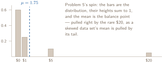
Interpreting them is the scored part. “” is a number; “over many plays, the game pays an average of $1.75 per play” is the interpretation, and “” becomes “a single play’s payout typically differs from that average by about $4.44.” Context and units, as the CED says, or the parameter has not been interpreted.
2. CHOOSE THE BOUNDARY
If , which complement gives : or ? Decide from the integers, not from the calculator.
7. THE BINOMIAL DISTRIBUTION: FOUR CONDITIONS, ONE FORMULA, TWO CALCULATOR FUNCTIONS
A binomial random variable counts successes in repeated trials when four things hold, and the exam asks you to check all four:
- binary — each trial is a success or a failure;
- independent — one trial’s outcome does not change another’s probability;
- fixed number of trials, , decided before you start;
- same probability of success, , on every trial.
Write . The probability of exactly successes is
where counts the arrangements of successes among trials and is the probability of any one arrangement. The mean and standard deviation need no table:
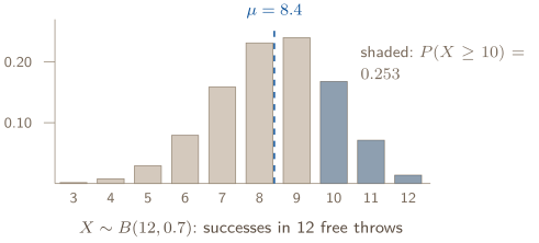
The boundary is an inequality, written first. “At least 10” is ; “more than 10” is ; “at most 7” is ; “fewer than 7” is . Write it in , then choose the tool: binompdf gives one value, binomcdf gives , and everything else is a complement — . The scored line is the inequality with the distribution named, not the keystrokes.
When it is not binomial. Drawing without replacement from a small population breaks independence (each draw changes the next ); counting trials until the first success has no fixed ; a probability that drifts across trials breaks the same- condition. The CED’s verb is justify why a random variable is or is not binomial: name the condition that fails.
CHECK 2 — CHOOSE THE BOUNDARY
. On a discrete variable the complement of “ or more” is “ or fewer”, and has to end up on exactly one side of the line. Numerically while , which is — a real answer to a question nobody asked, and it looks perfectly reasonable on the page. Write the inequality in first, then choose the button. The same one-step slip is why “more than ” is and not .
8. THE NORMAL DISTRIBUTION: SKETCH, SHADE, LABEL, STANDARDIZE
A continuous random variable takes any value in an interval, and probability is area: is the area under the density curve between and , the total area is , and the probability of any single exact value is — so and are the same number, unlike the binomial. A normal distribution, , is the continuous, unimodal, symmetric, bell-shaped curve fixed by its mean and standard deviation; a smaller makes it taller and narrower. The standard normal is , and moves any normal question onto it.
The empirical rule (68–95–99.7) estimates the area within one, two and three standard deviations; the table or the calculator gives the exact area for any boundary. The CED names four shapes of question, and each is a picture before it is a calculation:
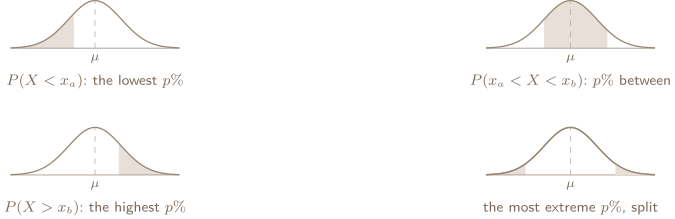
The routine, in the order the rubric wants it. Name the model, . Sketch the curve, mark and the boundary in the problem’s units, shade the region the words describe. Standardize: . Read the area — from the table, , so ; or from the calculator, normalcdf with the boundaries. Then the sentence. A percentile runs the routine backwards: the area is given, invert to (invNorm), then .
Comparing positions across two distributions. Two values from two normal models are compared by their -scores or their percentiles, never by their raw values — Unit 1’s z-score card, now with a curve behind it. The larger is the higher relative position. Extremeness in either direction is measured by ; a value far below the mean can be more extreme than one above it.
3. CHECK THE SAMPLING CONDITION
Does calling a sample “random” automatically make the exact standard deviation of its mean, when the sampling is done without replacement?
9. SAMPLING DISTRIBUTIONS, RANDOMIZATION DISTRIBUTIONS, AND THE CENTRAL LIMIT THEOREM
Every statistic — a sample mean, a sample proportion — would come out differently in a different sample. The sampling distribution of a statistic is the distribution of its values across all possible samples of size from the population. It is a distribution of statistics, not of data, and it has the same three properties as any distribution: a center, a spread, a shape.
For the sample mean of independent observations from a population with mean and finite standard deviation :
and the central limit theorem says its shape is approximately normal — better as grows — whatever the population’s shape. If the population is itself normal, the sampling distribution is exactly normal at every . The is the whole reason averaging works: a mean of 36 observations varies a sixth as much as one observation.
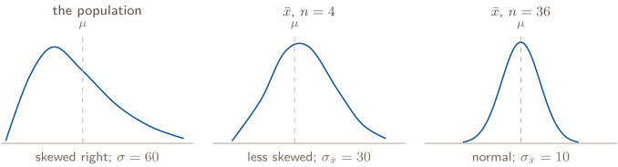
By simulation. Draw many random samples of size from a population with the parameter set to a known value, compute the statistic each time, and pile up the values: the pile approximates the sampling distribution. A randomization distribution does the same for an experiment: reassign the observed response values to the treatment groups at random, many times, computing the statistic each time — the distribution of a difference that chance alone would produce. Both are how Units 3 and 4 will decide whether an observed result is unusual.
Three sentences before a calculation. Center: minutes. Spread: minutes. Shape: approximately normal, by the central limit theorem, because is large. Then the normal routine of card 8, on .
CHECK 3 — CHECK THE SAMPLING CONDITION
No. The word “random” settles how the sample was chosen; is exact only when the observations are independent with the same variance, which is a different claim. Draw without replacement from a finite population and each draw changes what is left, so the observations are dependent and the true spread is slightly smaller than . The working rule is the condition: when the sample is no more than a tenth of the population, the dependence is small enough that is a fair approximation — and it is stated on the page, not assumed. Two habits fall out of this. Say which of the three sentences you are claiming and why; and never let a large stand in for a sound sample, because shrinks the spread around whatever the sampling method centred on, bias included.
PROBLEM 1
Two categorical variables: which total, and is there an association?
A random sample of 400 adults was asked whether they own an electronic reading device and how often they read for pleasure. The two-way table shows the results.
| reads daily | reads weekly | reads rarely | total | |
|---|---|---|---|---|
| owns a device | 72 | 56 | 32 | 160 |
| does not own one | 84 | 96 | 60 | 240 |
| total | 156 | 152 | 92 | 400 |
(a) Calculate the proportion of adults in the sample who own a device and read daily; the proportion who read daily; and the proportion of device owners who read daily. Name each kind of relative frequency. (b) Construct the conditional distribution of reading habit for owners and for non-owners, and display them in a segmented bar chart. (c) Is there an association between owning a device and reading habit in this sample? Justify. (d) A student says: “More non-owners read daily (84) than owners (72), so non-owners read more.” What is wrong with the comparison?
BEFORE YOU COMPUTE
Rung 1: data you have, two categorical variables, and the question is association. Before any division, write down which total answers which part — the grand total for a joint and a marginal proportion, the row total for a proportion of owners. Part (d) is the trap this problem exists for: the two rows have different sizes, so raw counts cannot be compared across them. Decide now that every comparison will be between conditional proportions.
WORKING
(a) Three divisions, three different totals.
The first is a joint relative frequency, a cell over the grand total. The second is a marginal relative frequency, a column total over the grand total. The third is a conditional relative frequency, the cell over its row total. Three questions about the same cell: how many of everyone are both; how many of everyone read daily; how many of the owners read daily.
(b) Each row divided by its own total.
| daily | weekly | rarely | |
|---|---|---|---|
| owners () | |||
| non-owners () |
Each row sums to , which is the check. The segmented bar chart is card 2’s figure: two bars to 100%, the daily segment 45% tall for owners and 35% for non-owners.
(c) Yes. The conditional distributions differ: among owners, 45% read daily and 20% rarely; among non-owners, 35% read daily and 25% rarely. Because the distribution of reading habit is not the same at both levels of ownership, the two variables are associated in this sample — owning a device goes with reading more often. That is a statement about these 400 adults; whether the association holds in the population, and whether ownership causes the reading, are different questions (Unit 5, and Unit 1’s design rules).
(d) The student compared counts from rows of different sizes: 240 non-owners against 160 owners. Eighty-four is more than seventy-two because there are more non-owners, not because non-owners read more. The fair comparison is the conditional proportion — against — and it runs the other way. Whenever groups differ in size, compare proportions, never counts.
ANSWER
(a) joint ; marginal ; conditional (b) owners ; non-owners (c) yes — the conditional distributions differ (45% against 35% daily) (d) counts from unequal groups; once conditioned
WATCH OUT
The wrong total. is the proportion of daily readers who own a device — a real number answering a different question from , the proportion of owners who read daily. “Of those who” and “among” point at the group whose total goes underneath; read the sentence for the group, then find its total. And in (c), “associated because the numbers are different” is not a justification; the justification names the conditional distributions and quotes two of their values.
CONNECTION
This table is the whole of Topics 2.4 to 2.7 in disguise: is , is , is , and independence means the full conditional distributions match. Equality for just the daily category tests independence of the two binary events; weekly and rarely must also be compared before concluding that the two variables are unassociated. Problem 3 reads the rules off this same table. And Unit 5’s chi-square test asks whether a difference like 45% against 35% is larger than sampling variation would produce in 400 people; the expected counts it compares against are the ones independence would give.
ABOUT THIS EXCERPT
This is the opening of a 36-page guide: the diagnostic tree, the full Master Toolbox, and the first worked problem. 7 more problems follow in the complete guide, each worked the same way — what to notice before you start, every step shown, and the mistake that problem invites. The complete guide is shared with families during the fit conversation.
Engineering Confidence — engineeringconfidence.one
Source and review notes
What this resource is
Complete browser edition of the public excerpt from an original Engineering Confidence AP Statistics unit-reference packet. All data sets and scenarios were created for this guide.
- Published
- Last reviewed
- Printable edition
- 18 pages
Course reference: official College Board course page.
Read this public excerpt above, or save the PDF for printing and offline reading.
Download the 18-page PDF excerpt