Read the public excerpt
The same instruction and worked examples appear here and in the printable PDF excerpt. You can request full guides for upcoming units below.
READ THIS FIRST
About this guide. Unit 1 asked one question of every situation: what is given up? Unit 2 puts that question inside a market. A demand curve is a row of buyers, each with a maximum they would pay; a supply curve is a row of sellers, each with a minimum they would accept. Where the rows meet, the price settles, the quantity settles, and every buyer who valued the good above the price and every seller who could make it below the price is better off by the difference. Everything else in the unit — elasticity, shifts, price controls, taxes, subsidies, tariffs — is a change to one of those rows and a reading of what happens to the meeting point and to the two areas beside it.
The graph is the answer format. On this unit the free-response section does not ask you to describe a market; it asks you to draw one, correctly labeled, and then to show a change on it. The College Board’s own note on the unit says students lose credit “for not properly labeling axes and curves on graphs and for not properly demonstrating the effects of changes on graphs.” Every figure in this guide is drawn the way a scored response has to be drawn — both axes named, both curves named, the shift as a second named curve with an arrow, the equilibria marked and read to both axes — so that the picture you copy into your own work is already a picture that scores.
The area is the reading. On the 2025 exam, 73% of students drew a subsidized market correctly and 8% could shade what the subsidy cost. Drawing is recall; reading is economics. Consumer surplus, producer surplus, deadweight loss, tax revenue and the cost of a subsidy are all areas on the graph you drew, and each has one correct shape. The habit this guide insists on: say which area it is, and why, before you shade it. Problems 5 to 9 do exactly that, every time.
Two calculations, done the wrong way more than any other. Elasticity is a ratio of percentage changes; the College Board names “the change in quantity divided by the change in price” as the error to expect, and Problem 3 shows why that number cannot be an elasticity. And surplus is the area of a particular triangle; the College Board’s other named error is students “calculate the area of the wrong triangle.” Problem 5 draws the right one and names the wrong ones beside it.
What this unit is worth. The Course and Exam Description puts Unit 2 at 20–25% of the multiple-choice section — with Unit 3, the heaviest weight in the course — and its graphs are the ones every later unit is built on. A four-function calculator is permitted on both sections.
Where each College Board topic lives in this guide.
2.1 Demand | the demand card; Problems 1, 2 |
|---|---|
2.2 Supply | the supply card; Problem 2 |
2.3 Price elasticity of demand | the elasticity-of-demand card; Problem 3 |
2.4 Price elasticity of supply | the elasticity-of-supply card; Problem 4 |
2.5 Other elasticities | the other-elasticities card; Problem 4 |
2.6 Market equilibrium and consumer and producer surplus | the equilibrium card; Problem 5 |
2.7 Market disequilibrium and changes in equilibrium | the changes card; Problems 5, 6 |
2.8 The effects of government intervention in markets | the intervention card; Problems 7, 8 |
2.9 International trade and public policy | the trade card; Problem 9 |
Diagnostic Decision Tree
How to use it. The pages that follow open with a decision tree for a problem you are about to start and a symptom map for one you are already inside. The Master Toolbox then defines the terms and methods the problems use; it is a reference, not assigned reading — open the card you need. Then, for each problem: read the prompt, read the “Before you compute” rail, and attempt the problem before reading the worked solution. If it is late and you are short on time, cover the “Working” section with your hand and predict its first line.
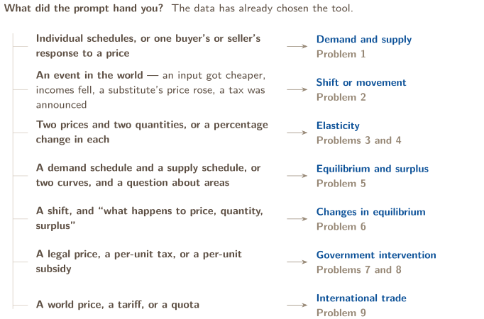
READ WHAT YOU WERE HANDED, BEFORE YOU READ THE QUESTION
Unit 2 has seven common routes, and the prompt signals one before it asks anything — in the shape of the data or the event it hands you. Sort on that first.
THEN THREE QUESTIONS, IN THIS ORDER
1. Did the price of this good change, or did something else change? A change in the good’s own price moves you along a curve and changes quantity demanded or supplied. Anything else that matters — income, a related good’s price, an input cost, expectations, the number of buyers or sellers, technology, a tax — shifts a curve and changes demand or supply. The vocabulary is the economics: “demand rose” and “quantity demanded rose” describe two different events, and the exam grades the difference.
2. Which curve does the event touch? Buyers’ circumstances shift demand; sellers’ costs and conditions shift supply. A tax on sellers shifts supply; a tax on buyers shifts demand; and — the surprise of Problem 8 — the market ends up in the same place either way.
3. What is the question actually asking for: a direction, a number, or an area? Explain wants the direction and the reason. Calculate wants a percentage change, an area of a triangle or a rectangle, with the arithmetic shown. Draw or show wants the labeled graph with the change on it. Decide before you start which of the three you owe, because they finish differently.
WHERE THE POINTS GO IN THIS UNIT
From the College Board’s own description of the unit, and the released scoring of the 2025 exam.
The graph, drawn to score. “Many students lose points on the AP Exam for not properly labeling axes and curves on graphs and for not properly demonstrating the effects of changes on graphs.” | Axes: price and quantity, with the good named. Curves: and , and or with an arrow for a shift. Equilibria marked and read to both axes. Problems 2, 6, 7. |
|---|---|
The area, named before it is shaded. 73% drew a subsidized market correctly; 8% shaded what the subsidy cost. | Consumer surplus is under demand, above price; producer surplus is above supply, below price; a tax’s revenue and a subsidy’s cost are rectangles, tax or subsidy by the new quantity; deadweight loss is the triangle between the curves over the lost trades. Say it, then shade it. Problems 5, 7, 8, 9. |
Elasticity as percentages. “…incorrectly calculate the elasticity of demand as the change in quantity divided by the change in price.” | , every time, with the two percentages written out. Problem 3. |
The right triangle. “…calculate the area of the wrong triangle.” | Height is the vertical distance from the price to the curve’s intercept; base is the quantity traded. Problem 5 draws the wrong ones too. |
Where to Look When You’re Stuck
HOW TO USE THIS MAP
The tree above is for a problem you are about to start. This table is for one you are already inside. Find the sentence that sounds like yours, do the move in the middle column, then open the card or problem on the right.
CURVES, SHIFTS, AND ELASTICITY
What is happening | First move | Where |
|---|---|---|
“I can’t tell whether the curve shifts or the point moves” | Ask whether the good’s own price changed. Own price: along the curve. Anything else: the curve moves. | p. 14, Prob. 2 |
“I don’t know which way to shift it” | Ask what happened to the quantity people want at every price. More at every price is right; less is left. Never reason from “up” and “down.” | p. 15, Prob. 2 |
“My elasticity is a huge number, or negative, or the same everywhere” | You divided changes, not percentage changes. Rebuild both percentages; report the magnitude and name the range. | p. 16, Prob. 3 |
“The question says total revenue” | Elastic: price and revenue move opposite ways. Inelastic: together. Unit: revenue is unchanged. | p. 16, Prob. 3 |
“Income or another good’s price changed and I’m asked for an elasticity” | The sign is the answer: income elasticity normal, inferior; cross-price substitutes, complements. | p. 17, Prob. 4 |
EQUILIBRIUM, AREAS, AND POLICY
What is happening | First move | Where |
|---|---|---|
“I have two schedules and need the equilibrium” | Find the price where ; or set the two equations equal and solve for , then read from either. | p. 18, Prob. 5 |
“I can’t tell which triangle is consumer surplus” | Under the demand curve, above the price paid, out to the quantity traded. Producer surplus is its mirror below the price. | p. 18, Prob. 5 |
“Both curves shifted and I can’t say what happens to price” | One of price and quantity is determinate from the directions alone; the other is indeterminate without magnitudes. Say which is which. | p. 20, Prob. 6 |
“A price ceiling or floor, and I’m not sure it does anything” | A ceiling binds only below equilibrium; a floor only above. Then read and at the legal price; the smaller one trades. | p. 22, Prob. 7 |
“A per-unit tax, and who pays it” | Shift the taxed side’s curve by the tax; the gap between the buyers’ price and the sellers’ price is the tax, and the less elastic side bears more of it. | p. 22, Prob. 8 |
“A world price, and the country imports or exports” | Below the domestic equilibrium the country imports the gap ; above it, exports . A tariff raises the domestic price by the tariff and shrinks the gap. | p. 24, Prob. 9 |
“I know the topic but still cannot find a first line” | Use the symptom list at the end of this guide. | final toolkit |
Master Toolbox — Everything These Problems Use
The cards below are independent reference tools. Start with the one the map named; no card assumes you read the one before it.
THE TASK VERB SETS THE RESPONSE JOB
The official verbs describe what a complete response must do.
Identify / What / Which / Will | Supply the requested information. No elaboration is required unless another part asks for it. |
|---|---|
Explain | State how or why the relationship, pattern, situation, or outcome occurs, using evidence or reasoning. A graph or symbol may be part of that explanation. |
Calculate | Show the mathematical steps that lead to the final answer, including units when the quantity has them. |
Draw a correctly labeled | Create the requested graph and include the labels needed to communicate its relationships — on this unit, both axes, both curves, and the equilibrium. |
Show / Label / Plot / Indicate | Put the requested scenario on the graph, with the new curve named, a directional arrow, and the new price and quantity read to the axes. |
On this unit the verb usually names an area or a direction. “Shade the deadweight loss” is a draw task; “explain what happens to consumer surplus” wants the direction and the reason; “calculate the tax revenue” wants a rectangle’s arithmetic on the page.
DEMAND: A ROW OF BUYERS, AND WHAT MOVES THEM
What the model assumes first. A market needs a well-defined system of property rights to function well — a seller can offer only what it owns and can transfer. Inside it, economic agents respond to incentives, and the price is the incentive this unit studies; but buyers also act under constraints — income, time, and the legal and regulatory frameworks around them — and the demand curve is what those incentives and constraints produce. The exam’s definitions of consumer decision making start there.
The law of demand. Other things equal, a higher price of a good lowers the quantity of it demanded; a lower price raises it. This is a movement along the demand curve, and the quantity that changes is called quantity demanded.
Why the curve slopes down — three reasons the exam accepts. The substitution effect: when the price rises, other goods look cheaper by comparison and buyers move toward them. The income effect: at a higher price a given income buys less, so buyers can afford less of everything, this good included. And diminishing marginal utility from Unit 1: each extra unit is worth less to a buyer, so a buyer takes an extra unit only at a lower price. Any one of them answers “explain why the demand curve is downward sloping”; the first two are the Course and Exam Description’s own words.
The demand curve is a marginal benefit curve. Read it vertically: at each quantity, the height of the curve is the most the marginal buyer would pay for that unit. That reading is what makes consumer surplus an area, and it is why the demand curve reappears in every later unit under the name .
Market demand is a horizontal sum. At each price, add every buyer’s quantity. The market curve is flatter than any one buyer’s, and it bends where a buyer drops out or enters. Problem 1 builds one.
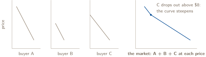
What shifts demand. Anything other than the good’s own price that changes how much buyers want at every price. Demand rises (the curve moves right) when buyers want more at each price; it falls (left) when they want less.
tastes and preferences | a fashion, a health finding, a season — right or left as they turn toward or away from the good |
|---|---|
income | for a normal good, more income shifts demand right; for an inferior good (bus rides, store-brand staples), more income shifts it left |
prices of related goods | a substitute’s price rising shifts this good’s demand right; a complement’s price rising shifts it left |
number of buyers | more buyers, more demand at every price |
expectations | a price cut expected next month shifts demand left now; an expected shortage shifts it right now |
The one thing that never shifts demand: the good’s own price. A price change moves the buyer along the curve that is already there. Writing “the price fell, so demand rose” describes a shift that did not happen; the sentence that scores is “the price fell, so quantity demanded rose.”
SUPPLY: A ROW OF SELLERS, AND WHAT MOVES THEM
The law of supply. Other things equal, a higher price raises the quantity supplied; a lower price lowers it — a movement along an upward-sloping supply curve. Read vertically, the supply curve is a marginal cost curve: at each quantity its height is the least the marginal seller would accept for that unit, because that is what the unit costs to make. Market supply is the horizontal sum of the sellers’ curves.
What shifts supply. Anything other than the good’s own price that changes what sellers will offer at every price. Supply rises (right) when producing is cheaper or easier; it falls (left) when producing is costlier.
input prices | cheaper labor, materials or energy shifts supply right; dearer inputs shift it left — the Course and Exam Description’s own example is “the price of alternative inputs” |
|---|---|
technology and productivity | a better method makes each unit cheaper: right |
number of sellers | more firms, more supply at every price |
prices of other goods the seller could make | if wheat pays better, corn supply shifts left — the seller’s own opportunity cost |
expectations | a seller expecting a higher price next month holds back today: left now |
taxes and subsidies | a per-unit tax shifts supply up by the tax (left); a per-unit subsidy shifts it down by the subsidy (right). Problem 8. |
Reading a shift as a vertical distance. A supply curve can move “left” or “up”; for a tax they are the same move. Up by $6 means: at every quantity, sellers now need $6 more to offer that unit. Thinking of supply shifts vertically is what makes taxes and subsidies easy to draw, so practice reading both ways.
PRICE ELASTICITY OF DEMAND: PERCENTAGES, OR IT IS NOT AN ELASTICITY
The definition. Price elasticity of demand measures how much quantity demanded responds to a price change, as a ratio of percentage changes:
The sign is always negative for a normal demand curve; report the magnitude and say which range it falls in.
| elastic — quantity moves by a larger percentage than price |
|---|---|
| inelastic — quantity moves by a smaller percentage |
| unit elastic — the same percentage |
| perfectly elastic — a horizontal demand curve; any price above the line sells nothing |
| perfectly inelastic — a vertical curve; the same quantity at any price |
The wrong number, named. — the change in quantity divided by the change in price — is the slope’s reciprocal. It has units (units per dollar), it is the same everywhere on a straight line, and it depends on whether you measured in thousands or in units. None of that can be true of an elasticity, which is a pure number that varies along the line. The College Board names this exact error as the one to expect. Write both percentages out before dividing and it cannot happen.
Which base? Unless the prompt says otherwise, use the percentage change from the initial values, as above. The midpoint method uses the average of the two values as the base for each percentage, over , and gives the same number whichever direction the price moved. Use it when the prompt asks for it, or names an arc elasticity; otherwise use the initial values and say so.
Slope is not elasticity. On a straight-line demand curve the slope never changes and the elasticity changes at every point: elastic in the upper half, unit elastic at the midpoint, inelastic in the lower half. Total revenue, , is a hill whose peak sits at that midpoint.
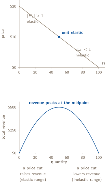
The total revenue test follows from the hill. If demand is elastic, price and total revenue move in opposite directions: a price cut raises revenue. If demand is inelastic, they move together: a price cut lowers revenue, and a price rise raises it. For a finite change measured with midpoint elasticity, unit elasticity means unchanged revenue. With two exact price–quantity pairs, checking directly is decisive. An initial-value percentage calculation can classify a large interval differently: from to its magnitude is 1.5, yet revenue is $480 at both ends. This is how the exam usually asks about elasticity without saying the word — “the store cut its price and its revenue rose; what does that tell you about demand?”
What makes demand elastic. The availability of close substitutes is the one the Course and Exam Description names; a good with many substitutes is elastic because buyers can leave. Also: a larger share of the buyer’s budget (more elastic), a luxury rather than a necessity (more elastic), and more time to adjust (more elastic in the long run).
PRICE ELASTICITY OF SUPPLY, AND THE OTHER ELASTICITIES
Supply. The same ratio, on the sellers’ side:
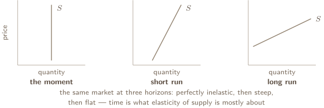
positive, with the same benchmarks: elastic above 1, inelastic below, unit at 1, perfectly elastic horizontal, perfectly inelastic vertical. What makes supply elastic is how easily sellers can change output: spare capacity, movable inputs, and above all time — supply is nearly vertical in the moment (the concert is tonight; the seats are the seats), steep in the short run, and flat in the long run when new sellers can enter. The Course and Exam Description’s named factor is “the price of alternative inputs”: if the seller can switch to a cheaper input as it expands, supply is more elastic.
Income elasticity of demand measures how quantity demanded responds to a change in buyers’ income:
| a normal good; above 1, often called a luxury |
|---|---|
| an inferior good |
Cross-price elasticity of demand measures how the quantity of one good responds to the price of another:
| substitutes — got dearer, buyers moved to |
|---|---|
| complements — got dearer, less was used with it |
| unrelated |
For these two, the sign is the answer. Price elasticity of demand is reported as a magnitude because its sign is always the same; income and cross-price elasticities are reported with their sign because the sign is the classification the question is after. Compute the number, keep the sign, then name the good. Problem 4 does all three.
MARKET EQUILIBRIUM, AND THE TWO AREAS BESIDE IT
Equilibrium is the price at which quantity demanded equals quantity supplied — the market clears: every buyer willing to pay the price finds a seller, every seller willing to accept it finds a buyer, and there is neither a shortage nor a surplus. In a competitive market with no failures, that price and quantity are efficient: no other quantity creates more total surplus.
Finding it. From two schedules, scan for the price where the quantities match. From two equations, set them equal and solve: with demand and supply , gives and . Check by putting into both equations; if they disagree, the algebra slipped.
Consumer surplus is what buyers gained: for every unit, the most its buyer would have paid minus what was actually paid, summed. On the graph that is the area under the demand curve, above the price, out to the quantity traded. Producer surplus is the mirror: what sellers received minus the least they would have accepted — above the supply curve, below the price, out to the quantity traded. Their sum is total economic surplus, the whole gain the market creates.
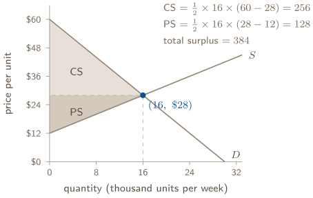
The triangle’s dimensions, said precisely. Base is the quantity traded, along the axis. Height is a vertical distance on the price axis: from the price up to the demand intercept for CS, from the price down to the supply intercept for PS. Both areas are in dollars (quantity dollars per unit), and if the quantity axis is in thousands, so is the area. With schedules rather than lines, sum the per-unit gaps instead; Problem 5 does both.
What the price is for. The equilibrium price is information. It tells every buyer and seller what a unit is worth at the margin, and resources move toward the uses where that signal says they are valued most: a price that rises after a demand shift is not only an outcome, it is the instruction that pulls more inputs into making the good. That is why the Course and Exam Description says the equilibrium price “provides information to economic decision-makers to guide resource allocation.”
Why equilibrium is efficient. Every unit up to 16 has a buyer who values it above the seller’s cost — the demand curve is above the supply curve — so trading it adds to total surplus. The 17th unit would cost more to make than any remaining buyer would pay, so trading it would subtract. Total surplus therefore peaks exactly where the curves cross, and any policy that moves the quantity away from it, in either direction, throws some of that surplus away. That thrown-away amount has a name in the next cards: deadweight loss.
A check first. One question opens three of the pieces below and is answered where that piece ends. Answer it before you read on. Getting it wrong is the point — that is what makes it stick.
1. CHOOSE WHAT IS DETERMINATE
Demand and supply both increase. Which equilibrium change is determined without knowing the sizes of the two shifts?
DISEQUILIBRIUM, AND CHANGES IN EQUILIBRIUM
A price that is not the equilibrium price. Above it, sellers offer more than buyers take: a surplus of , and unsold goods push the price down. Below it, buyers want more than sellers offer: a shortage of , and unmet buyers bid the price up. Market forces drive the price back to equilibrium unless something holds it away — which is what a price control does. Read and off the two curves at the stated price; the difference is the surplus or shortage, and the smaller of the two is what actually trades.
One curve shifts. Four cases, and each has a determinate answer for both price and quantity.
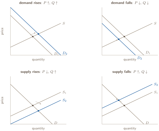
Read them as a rule rather than four pictures: a demand shift moves price and quantity the same way; a supply shift moves them opposite ways. Which way is decided by whether the curve moved right (more at every price) or left.
Both curves shift. Now one of the two outcomes is determinate from the directions alone and the other depends on how far each curve moved.
shifts | quantity | price |
|
|---|---|---|---|
right, right | rises | indeterminate | both push up; they pull opposite ways |
left, left | falls | indeterminate |
|
right, left | indeterminate | rises | both push up; they pull opposite ways |
left, right | indeterminate | falls |
|
On the exam, “indeterminate” is a full-credit answer when you say why: “price could rise, fall, or stay the same, depending on the relative sizes of the shifts.” Guessing a direction is the way to lose the point. If the prompt gives magnitudes, the numbers decide, and Problem 6(c) is a case where they land the price exactly where it started.
Surplus moves with the shift. A rightward demand shift raises price and quantity, so producer surplus rises for certain; consumer surplus usually rises too, because the shift itself means buyers value the good more. A rightward supply shift lowers price and raises quantity, so consumer surplus rises for certain. How much price moves depends on elasticity: the same demand shift raises price more against a steep, inelastic supply than against a flat one, because sellers cannot expand to meet it. Problem 6(d) puts numbers on that.
CHECK 1 — CHOOSE WHAT IS DETERMINATE
Quantity. Both shifts push quantity the same way — more demand raises it, more supply raises it — so quantity rises whatever their sizes. Price is the indeterminate one: demand pulls it up, supply pushes it down, and which wins depends on which shift is larger. The rule is not a list to memorise: whichever variable both curves agree about is determined, and the other one is not. “Indeterminate” is the full-credit answer when you say why.
2. SEPARATE WILLINGNESS FROM TRADE
A binding price ceiling leaves quantity demanded at 100 and quantity supplied at 60. In the basic model, with no black market, are 100 units traded?
GOVERNMENT INTERVENTION: PRICE CONTROLS, TAXES, SUBSIDIES
Every intervention on this card holds the market away from the quantity where the curves cross, and the cost of doing so has the same name each time: deadweight loss, the surplus from the trades that no longer happen. Read every case in the same order — where is the new quantity, what price do buyers pay, what price do sellers keep, and which areas changed.
A price ceiling is a legal maximum. It binds only if it is below the equilibrium price; a ceiling above equilibrium changes nothing. Binding, it creates a shortage: at the low price buyers want more and sellers offer less, and the quantity that actually trades is the smaller number, . Rent control is the exam’s favorite example.
A price floor is a legal minimum. It binds only if it is above equilibrium, and then creates a surplus: sellers offer more than buyers take, and the quantity traded is . A minimum wage is the example, with labor as the good.
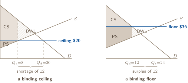
In both pictures the quantity traded fell from 16, and the hatched triangle is the surplus those lost trades would have created. Some surplus also moved: under the ceiling, buyers who still get the good pay less, so a rectangle of producer surplus became consumer surplus; under the floor, the reverse. Problem 7 computes every area.
A per-unit tax drives a wedge between what buyers pay and what sellers keep, equal to the tax. Draw it as a shift of the taxed side’s curve by the amount of the tax: a tax on sellers shifts supply up by (sellers need more per unit); a tax on buyers shifts demand down by . Either way the market lands in the same place — statutory incidence, who writes the check, does not decide economic incidence, who bears the cost. Then:
quantity | falls to where the shifted curve meets the other one |
|---|---|
buyers’ price | read off the demand curve at the new quantity |
sellers’ price | buyers’ price minus the tax; equivalently, off the original supply curve at the new quantity |
tax revenue | the rectangle: tax new quantity |
deadweight loss | the triangle between and the original from the new quantity to the old one |
incidence | the side with the less elastic curve bears more of the tax — it is the side that cannot get out of the way |
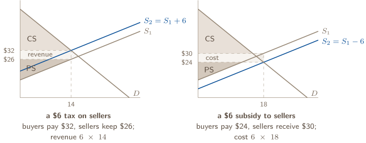
A per-unit subsidy is the tax run backwards: supply shifts down by the subsidy, quantity rises past the efficient one, buyers pay less and sellers receive more, and the gap between them is the subsidy. The cost to the government is the rectangle subsidy new quantity — the area 92% of students could not shade in 2025. Buyers and sellers gain, but less than the subsidy costs, and the shortfall is the deadweight loss: the extra units cost more to make than they were worth.
Quantity controls. A quota caps the quantity below the equilibrium one; price rises to what buyers will pay for that smaller quantity, and the surplus from the lost trades is deadweight loss. The Course and Exam Description keeps the graphing of quotas out of scope but the quantity reasoning in.
The line that earns the efficiency point. A tax, a subsidy, a ceiling, a floor or a quota placed on a market that was producing the efficient quantity reduces allocative efficiency when it changes quantity away from that efficient level. First check whether the policy binds and whether quantity changes. A nonbinding price control has no effect; deadweight loss measures surplus lost on affected trades.
CHECK 2 — SEPARATE WILLINGNESS FROM TRADE
No — 60 trade. Willingness to buy is not the same thing as a trade: a trade needs a buyer and a seller, so the quantity exchanged is the smaller of the two, the short side of the market. The 40-unit gap is the shortage, and it is a quantity nobody supplies rather than a quantity someone buys. Read the smaller number off the two curves at the controlled price, every time.
INTERNATIONAL TRADE: A WORLD PRICE, AND A TARIFF
Autarky is the closed economy: the domestic equilibrium of the earlier cards. Opening to trade means the domestic price becomes the world price, drawn as a horizontal line, and the gap between what domestic buyers want and domestic sellers offer at that price is filled by trade.
world price below the domestic equilibrium | the country imports . Buyers gain (a lower price, more bought); domestic sellers lose (a lower price, less sold); total surplus rises, so the country as a whole gains. |
|---|---|
world price above it | the country exports . Sellers gain, domestic buyers lose, total surplus rises. |
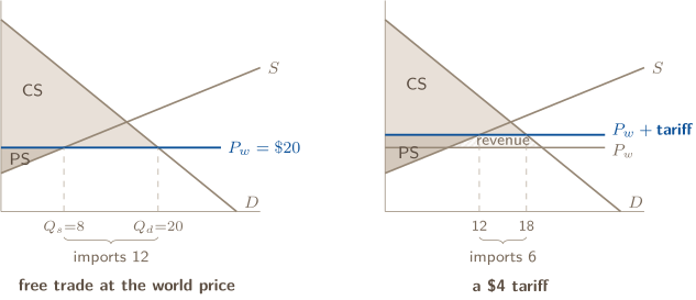
A tariff is a tax on imports. It raises the domestic price by the tariff, so domestic sellers offer more and domestic buyers take less: the import gap shrinks. Read the areas in this order — consumer surplus falls (the price rose); producer surplus rises (domestic sellers sell more at more); the government collects tariff the imports that remain, the rectangle over the gap; and two hatched triangles are deadweight loss, one for the units now made at home at more than the world price, one for the units buyers no longer buy. Problem 9 computes all five.
A quota limits the import quantity directly. It raises the domestic price the same way a tariff of the right size would, but the rectangle goes to whoever holds the import licenses rather than to the government. The Course and Exam Description keeps the quota’s graph out of scope and its quantity effect in.
PROBLEM 1
Three buyers, one market: building demand from the people in it
A campus coffee cart serves three regular buyers. The table shows how many iced coffees each would buy per week at each price:
| price per coffee | $2 | $4 | $6 | $8 | $10 |
|---|---|---|---|---|---|
| Asha | 10 | 8 | 6 | 4 | 2 |
| Ben | 6 | 5 | 4 | 3 | 2 |
| Cora | 9 | 6 | 3 | 0 | 0 |
(a) State the law of demand, and give two reasons the College Board accepts for why an individual’s demand curve slopes downward. (b) Build the market demand schedule. (c) Draw a correctly labeled graph of the market demand curve. (d) The cart cuts its price from $6 to $4. What happens to the quantity demanded, and what happens to demand? (e) A fourth regular, Dev, starts buying: 5 coffees at every price from $2 to $10. What happens to demand now, and by how much?
BEFORE YOU COMPUTE
The table is three individual schedules. The market is not a fourth person; it is the three of them added up at each price, one price at a time. Read down a column, not along a row.
Parts (d) and (e) are the vocabulary test of the whole unit, and they are placed next to each other on purpose. One is a change in the good’s own price. The other is a change in something else. Decide which is which before you write a word, because the two events have different names and the exam grades the name.
WORKING
(a) The law, and the reasons. Other things equal, when the price of a good rises the quantity demanded falls, and when the price falls the quantity demanded rises. Two reasons: the substitution effect — at $8 a coffee, tea and the vending machine look cheaper by comparison, so some coffees are replaced — and the income effect — at $8 the same weekly budget buys fewer things altogether, coffee among them. A third, from Unit 1: each extra coffee in a week is worth less to the drinker than the last, so a buyer takes another only at a lower price.
(b) The market schedule. Add down each column.
| price | $2 | $4 | $6 | $8 | $10 |
|---|---|---|---|---|---|
| Asha + Ben + Cora | |||||
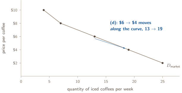
| market quantity demanded | 25 | 19 | 13 | 7 | 4 |
Notice the pattern in the differences: 6, 6, 6, then 3. Between $2 and $8 every step of $2 loses six coffees; between $8 and $10 it loses three, because Cora has already stopped buying at $8 and only two buyers are left to respond. The market curve is a sum, and it bends where a buyer leaves.
WORKING
(c) What the graph must carry. Price on the vertical axis, quantity on the horizontal, both labeled with what they measure; the curve named ; the plotted points at the schedule’s prices. That is the whole task when the verb is draw.
(d) The price cut. The good’s own price changed, so this is a movement along the curve that is already there: quantity demanded rises from 13 to 19 coffees a week. Demand did not change. The curve is exactly where it was; the cart is at a different point on it. The sentence that scores: “the lower price increases the quantity demanded; demand is unchanged.”
(e) A fourth buyer. Nothing happened to the price. Something happened to who is in the market, and that changes the quantity wanted at every price: the market schedule becomes 30, 24, 18, 12, 9. This is an increase in demand — the whole curve shifts right by five coffees at every price. On a graph, draw the new curve, name it , and put an arrow from to .
ANSWER
(a) Quantity demanded falls as price rises, other things equal; because of the substitution effect and the income effect (and diminishing marginal utility). (b) 25, 19, 13, 7, 4 at $2, $4, $6, $8, $10. (c) A downward-sloping curve through those points, axes labeled price and quantity, curve labeled . (d) Quantity demanded rises from 13 to 19; demand is unchanged — a movement along the curve. (e) Demand increases: the curve shifts right by 5 at every price, to 30, 24, 18, 12, 9.
WATCH OUT
Adding along a row. is one buyer’s quantities at five prices summed, which means nothing. The market is a sum across buyers at one price: read down.
“The price fell, so demand rose.” This is the sentence the exam is built to catch. A change in the good’s own price never shifts its demand curve. If you find yourself writing “demand rose” after a price change, replace it with “quantity demanded rose” and check whether the meaning survives. It does, and it is now correct.
Drawing the market curve straight. It is not straight, because a buyer dropped out. A student who “smooths” it has drawn a different schedule. Plot the points; connect them; let the bend stand.
CONNECTION
Supply is built the same way, one seller at a time, and its curve is read the same way: a change in the good’s own price moves the seller along it, anything else moves the curve. Problem 2 sorts eight events into those two bins, for both curves at once.
ABOUT THIS EXCERPT
This is the opening of a 50-page guide: the diagnostic tree, the full Master Toolbox, and the first worked problem. 8 more problems follow in the complete guide, each worked the same way — what to notice before you start, every step shown, and the mistake that problem invites. The complete guide is shared with families during the fit conversation.
Engineering Confidence — engineeringconfidence.one
Source and review notes
What this resource is
Complete browser edition of the public excerpt from an original Engineering Confidence AP Microeconomics unit-reference packet. Every problem and scenario was written for this guide.
- Published
- Last reviewed
- Printable edition
- 22 pages
Course reference: official College Board course page.
Read this public excerpt above, or save the PDF for printing and offline reading.
Download the 22-page PDF excerpt