Read the public excerpt
The same instruction and worked examples appear here and in the printable PDF excerpt. You can request full guides for upcoming units below.
READ THIS FIRST
About this guide. Most students meet economics as vocabulary — a list of terms to define, a curve to memorize the name of. That version of the subject is nearly impossible to be good at, because the definitions all sound reasonable and none of them tell you what to do when a problem lands in front of you.
Unit 1 is where the other version starts. Economics is a modeling discipline: you are handed a constrained system, you build the smallest model that captures the constraint, and you read the answer off the model. The ideas here share one spine.
Scarcity starts the chain. Limited resources force individuals and societies to choose; an economic system supplies the institutions and coordinating mechanism for making and distributing those choices. An opportunity cost then puts a value on the next-best alternative forgone. The production possibilities curve displays those trade-offs; comparative advantage compares them; marginal analysis asks whether one more unit is worth its cost; and consumer choice applies that comparison under a budget. The recurring question is: what is constrained, what is the available alternative, and what is given up?
That is why the guide is fussy about two things that look like housekeeping.
Units, on every calculation. An opportunity cost should never be an unlabeled number. It may be dollars or hours; when both alternatives are goods, it is a rate — 0.8 trailers per bike, 2 sensors per drone, 4 stools per cabinet. Students who write “the opportunity cost is 0.8” have left the answer ambiguous. Carry the units and the arithmetic corrects you: if you divide the wrong way, the units come out upside down and you can see it before finishing.
The graph is an answer format, not an illustration. On the free-response section, drawing is a scored task in its own right — the College Board’s own exam description puts the “create graphs or visual representations” task at 30–50% of the free-response points. The Toolbox entry “The graph as an answer format” is a compact completeness checklist; run it every time a question says draw.
What this unit is worth. The College Board’s Course and Exam Description puts Unit 1 at 12–15% of the multiple-choice section — one of the lighter units by weight, and by a distance the most load-bearing, since Units 2 through 6 are built entirely out of it. A four-function calculator is permitted on both sections, so the arithmetic here is meant to be done, not estimated.
Where each College Board topic lives in this guide.
1.1 Scarcity | the scarcity card; Problem 9(a) |
|---|---|
1.2 Resource allocation and economic systems | the economic-systems card; Problem 9(d)(e) |
1.3 Production possibilities curve | the four PPC cards; Problems 2, 3, 9(b)(c) |
1.4 Comparative advantage and trade | the advantage, tables and terms-of-trade cards; Problems 4, 5, 6 |
1.5 Cost-benefit analysis | the opportunity-cost and totals cards; Problems 1, 7 |
1.6 Marginal analysis and consumer choice | the marginal and consumer-choice cards; Problems 7, 8 |
Diagnostic Decision Tree
How to use it. The pages that follow open with a decision tree for a problem you are about to start and a symptom map for one you are already inside. The Master Toolbox then defines the terms and methods the problems use. Treat it as a reference: the map tells you which card or worked problem to open, so there is no need to read every card before Problem 1.
Then, for each problem: read the prompt, read the “Before you compute” rail, and attempt the problem before reading the worked solution. Reading a solution you have not struggled with feels like learning and mostly is not. If it is late and you are short on time, cover the “Working” section with your hand and predict its first line; even that much turns reading back into thinking.
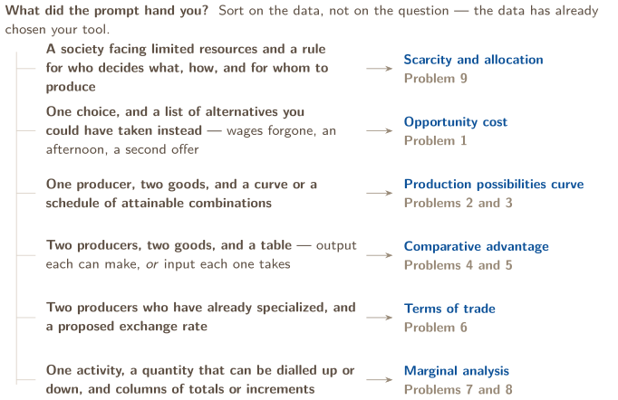
READ WHAT YOU WERE HANDED, BEFORE YOU READ THE QUESTION
Unit 1 has six common routes, and the prompt usually signals one before it asks you anything — not only in the question, but in the shape of the situation or data it hands you. Learn to sort on that and you stop guessing.
THEN THREE QUESTIONS, IN THIS ORDER
1. What is being given up? Ask it before you write anything. For any quantitative trade-off in this unit, if you cannot name what is being surrendered you are not yet solving the problem. In a PPC question it is the good on the other axis. In a trade question it is the good the producer stops making. In a marginal question it is whatever the next dollar or hour would otherwise have bought. Name it out loud, with its units, before computing.
2. Is the table telling me output or input? This one question decides whether your ratio goes one way or the other, and it is one of the easiest places to invert an otherwise sound solution. An output table says how much a producer makes from a fixed amount of resource: “24 sensors or 12 drones per worker-day.” An input table says how much resource one unit consumes: “8 labor-hours per cabinet.” They contain the same information and the arithmetic runs in opposite directions. Problems 4 and 5 are the same question asked both ways, deliberately.
Read the column heading, not the numbers. If the heading has a good in it (“sensors per worker-day”), it is output. If the heading has a resource in it (“labor-hours per cabinet”), it is input.
3. Am I being asked about a total, or about one more? Totals and margins answer different questions and routinely disagree. “Is this project worth doing at all?” is a total question — compare total benefit with total cost. “How much of it should we do?” is a marginal question — compare the benefit of the next unit with the cost of that same unit, and stop when they meet. Answering a marginal question with totals or with averages produces a confident, specific, wrong number; Problem 7 shows exactly which one.
And when the question says “draw”: that is not a request for a picture beside your answer. The requested relationships and labels belong in the visual itself. See “The graph as an answer format” in the Toolbox before you attempt Problem 3.
WHERE THE POINTS GO IN THIS UNIT
The College Board’s own description of this unit names where students lose credit. Four habits, each earned in a problem below, cover nearly all of it.
The graph, drawn to score. “Graphing is an important skill in this course that will be tested in the free-response section … stressing the importance of properly labeling axes and curves.” | Axes carry the goods and the period; every curve is named; a change is a second curve and an arrow; a referenced point is marked. Problems 3(e) and 9(c). |
|---|---|
The calculation, shown. “Students should understand the importance of showing their work when doing any calculations.” | The units chain on the page, the answer with its units. A bare 0.8 is not a calculation. Problems 2 to 6. |
Consumer choice, with numbers. “Many students grasp the concept of consumer optimization, [but] are unable to apply that understanding using numbers.” | Marginal utility per dollar, computed for every unit, and the feasible bundles compared. Problem 8. |
The verb, obeyed. Identify wants the item; explain wants the how or why; calculate wants the steps; draw wants the labeled visual. | Read the verb before the economics. The task-verb card opens the Toolbox. |
Where to Look When You’re Stuck
HOW TO USE THIS MAP
The tree above is for a problem you are about to start. This table is for one you are already inside. Find the sentence that sounds like yours, do the move in the middle column, then open the card or problem on the right. The Master Toolbox is a reference, not assigned reading.
CHOICES, CURVES, AND TRADE
What is happening | First move | Where |
|---|---|---|
“There are more wants than the available resources can satisfy” | Name the scarce factors, then ask who coordinates what, how, and for whom. | p. 14, Prob. 9 |
“There are several alternatives and I keep adding them” | Choose the single next-best alternative; do not sum mutually exclusive options. | p. 15, Prob. 1 |
“I cannot tell whether the point is efficient” | Compare it with the frontier at the same coordinate; then name on, inside, or outside. | p. 19, Prob. 2 |
“The PPC is straight, bowed, or moving” | Compute opportunity cost over two segments, then separate a capacity change from a product-mix change. | p. 20, Prob. 3 |
“The table gives hours instead of goods” | Build a units chain. Resource per good is an input table; smaller input is stronger. | p. 25, Prob. 4–5 |
MARGINS, BUNDLES, AND ANSWER FORM
What is happening | First move | Where |
|---|---|---|
“My terms-of-trade range is backwards or empty” | Put the exporter’s opportunity cost at the floor and the importer’s at the ceiling; use strict bounds only for strict gains to both. | p. 26, Prob. 6 |
“Totals and margins recommend different quantities” | First identify the alternatives still available. For an incremental choice, compare the next unit’s MB with its MC. | p. 28, Prob. 7 |
“My utility ratios do not become equal” | Ask whether goods are divisible. With whole units, compare feasible bundles and rule out any affordable utility-improving reallocation. | p. 30, Prob. 8 |
“The prompt says explain, calculate, or draw” | Let the verb set the response job: reasoning, shown mathematical steps, or a fully labeled visual. | p. 12, Prob. 3, 9 |
“I know the topic but still cannot find a first line” | Use the symptom list at the end of this guide. | final toolkit |
Master Toolbox — Everything These Problems Use
The cards below are independent reference tools. Start with the one the map named; no card assumes you read the one before it.
THE TASK VERB SETS THE RESPONSE JOB
The official verbs describe what a complete response must do; they do not promise a particular point or require the same finishing move on every question.
Identify / What / Which / Will | Supply the requested information. No elaboration is required unless another part asks for it. |
|---|---|
Explain | State how or why the relationship, pattern, situation, or outcome occurs, using evidence or reasoning. A graph or symbol may be part of that explanation. |
Calculate | Show the mathematical steps that lead to the final answer, including units when the quantity has them. |
Draw a correctly labeled | Create the requested graph or visual and include the labels needed to communicate its relationships. |
Show / Label / Plot / Indicate | Put the requested scenario on the student-created visual, with axes, curves, labels, and directional changes where relevant. |
The verb and the economics work together. A numerical result can support an explanation, but the number alone does not explain; a sentence can interpret a graph, but it does not replace labels the prompt asked the student to draw.
THE STARTING CONDITION: SCARCITY
Resources (also called factors of production) are the inputs an economy has to work with. The Course and Exam Description gives land (natural resources), labor (human effort), and capital (tools, machines, buildings — things made in order to make other things) as examples, not as an exhaustive list. Many economics courses also name entrepreneurship: the organizing, innovation, and risk-taking that combines the other factors. Follow the convention a prompt establishes, and do not treat a four-factor list as a contradiction.
Scarcity is the condition that resources are limited while wants are not. It is not the same as a shortage, which is a temporary market condition you will meet in Unit 2. Scarcity is the reason the subject exists: if resources were unlimited, nothing would have to be given up, and every idea in this guide would be empty.
One exception, and the exam knows about it. Most factors of production are scarce — but not all. Some are non-rival, meaning one person’s use of them does not reduce what is left for anyone else. Established knowledge is the standard example: if you use the Pythagorean theorem today, there is not less of it tomorrow, and my using it does not consume your access to it. Land, labor, and a given machine are all rival — an hour of a welder’s time spent on bikes is gone from trailers — and that rivalry is what creates opportunity cost. So state the general claim carefully: most resources are scarce, and it is the scarce, rival ones that force the trade-offs this unit is about.
Because resources are scarce, every economy has to answer three questions: what to produce, how to produce it, and who gets what is produced. The arrangement a society uses to answer them is its economic system — a command economy answers them centrally, a market economy answers them through voluntary exchange and prices, and a mixed economy uses both. The next card sets the three side by side, because the exam asks for their differences and their limits, not their names.
A trade-off is what scarcity produces at the level of a single decision: to have more of one thing you must accept less of another. When you put a number on a trade-off, you have an opportunity cost.
RESOURCE ALLOCATION AND ECONOMIC SYSTEMS
Every society must answer three questions, and an economic system is the set of institutions and the coordinating mechanism it uses to answer them. The exam’s verb here is usually explain or identify: which mechanism a described arrangement uses, how it settles each question, and what it cannot do well.
| command | market | mixed |
|---|---|---|---|
coordinating mechanism | a central authority’s plan | prices, formed by voluntary exchange | both, in different sectors or layers |
what to produce | the planner’s priorities | what buyers will pay for | markets, with public provision of some goods |
how to produce | assigned inputs and methods | whichever method the producer finds cheapest | producers choose, within regulation |
for whom | rationing, queues, rank | willingness and ability to pay | pay, plus transfers and entitlements |
one limitation | the planner lacks dispersed, changing local information | ability to pay need not track need | the boundary between the two is itself contested |
Property rights and enforceable contracts are what let the market mechanism work at all — a price cannot coordinate anything nobody can hold or trade. Every real economy is mixed; the useful question in a prompt is which mechanism is doing the work in this arrangement, not which label the whole country wears. Problem 9 gives three arrangements and asks exactly that.
OPPORTUNITY COST: THE DEFINITION, SAID PRECISELY
The opportunity cost of a choice is the value of the next-best alternative you gave up to make it.
Three words in that sentence do real work, and each prevents a different misreading.
“Next-best” — singular. If you could have chosen one of three mutually exclusive uses of the same resource, the opportunity cost is the single most valuable one, not their sum. You were only ever going to do one of them, so only one was truly given up. If alternatives can be combined, first define the actual feasible choices rather than applying this shortcut.
“Alternative” — the thing forgone, not the thing chosen. It is measured in whatever the alternative would have delivered: dollars, hours, sensors, stools.
“Value” — not price. What the alternative was worth to the person choosing.
Explicit and implicit costs. An explicit cost is money that actually leaves your hands — parts, rent, a permit. An implicit cost is the value of a resource you already own and used up anyway: your own time, a building you already own, savings you spent instead of leaving invested. Implicit costs never appear on a receipt, which is precisely why people forget them, and why the exam tests them.
Two profits, and they answer different questions.
accounting profit | revenue explicit costs. What a tax form sees. |
|---|---|
economic profit | revenue explicit costs implicit costs. What tells you whether the choice was worth making. |
Economic profit is never larger than accounting profit — implicit costs cannot be negative — and the gap between the two is exactly the value of the implicit costs counted in the decision. They are equal exactly when implicit cost is zero; explicit costs may still be positive. A venture can post a healthy accounting profit and a negative economic profit at the same time; that combination means it made money and still was not worth doing, because something else would have paid better. Problem 1 is that situation, in dollars.
A check first. One question opens three of the cards below and is answered at that card’s end. Answer it before you read on. Getting it wrong is the point — that is what makes the card stick.
1. ORIENT THE RATIO
With the same resources a producer can make 6 shirts or 3 tables. What is the opportunity cost of one shirt? Explain what belongs in the numerator.
OPPORTUNITY COST AS A RATIO — AND WHY YOU CARRY THE UNITS
When both the thing gained and the thing given up are goods, opportunity cost is a rate: how much of one good per one unit of the other. Write it that way every time.
You never have to remember which number goes on top. Build the rate as a chain of conversions and let the units cancel, the way you would in chemistry or physics. If a worker-day produces either 24 sensors or 12 drones, then:
“Worker-day” appears once on top and once on the bottom, so it cancels, and what survives is sensors per drone — which is exactly what an opportunity cost of a drone should be measured in. Set the chain up so the units cancel and the arithmetic cannot come out inverted.
The reciprocal check. For any one producer, the two opportunity costs are reciprocals:
Two sensors per drone and one-half drone per sensor: . Do this check on every pair you compute — it costs five seconds and catches an inverted ratio instantly. If your two numbers do not multiply to 1, one of them is upside down. It catches one inversion, though, not two: flip both and the product is still 1. That is why the units sentence below is the check that finishes the job.
Say the units out loud. “The opportunity cost is 0.8” is not an answer; 0.8 of what, per what? “0.8 trailers per bike” is an answer, and it also tells you the direction — bikes are what you are getting, trailers are what you are paying.
CHECK 1 — ORIENT THE RATIO
Half a table. The numerator is what you give up: 3 tables surrendered over 6 shirts gained, so tables per shirt. The units are the whole answer and they are also the check — say it aloud as “tables given up per shirt gained” and an upside-down ratio announces itself, because “2 shirts per table” is the answer to the other question. Getting a number without its units means you cannot tell which question you answered.
THE PRODUCTION POSSIBILITIES CURVE
A production possibilities curve (PPC) shows every combination of two goods a producer can make when all of its resources are fully employed and its technology is fixed. It is the simplest complete model in the course: two axes, one curve, and everything the model has to say is in the curve’s position and shape.
Where a point sits relative to the curve is the whole of the reading.
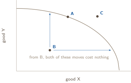
A | On the curve — efficient. Every resource is employed and employed well. From here, more X is available only by accepting less Y: the trade-off is live, and the opportunity cost is positive. |
|---|---|
B | Inside the curve — attainable but inefficient. Resources are idle (unemployment) or misallocated. The diagnostic signature is the two blue arrows: there are Pareto-improving paths on which the producer gets more of at least one good without giving up any of the other. Those particular moves have zero opportunity cost. That does not make every move from an interior point free; moving from B toward an endpoint can still require sacrificing the other good. Inefficiency means some mutually improving reallocation remains available. |
C | Outside the curve — unattainable. Not with today’s resources and today’s technology. No reallocation reaches it; the curve itself has to move. |
THE SLOPE’S MAGNITUDE IS THE OPPORTUNITY COST — SO THE SHAPE IS THE STORY
Moving rightward along a downward-sloping PPC, the numerical slope is negative while opportunity cost is a positive amount forgone. Therefore
when the axes increase in the usual directions. The curve’s shape is a statement about how that magnitude behaves.
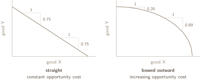
Both panels show the same measurement taken twice: advance one unit along the horizontal axis, read how far the curve falls. The straight PPC drops the same amount in both places; the bowed one drops further the second time, which is what “each additional X costs more Y than the one before” looks like.
Why a PPC bows outward. Because resources are not equally suited to both goods. Start at the top of the curve, making only Y. To make your first few X, you move over the resources that were worst at Y and best at X — you lose almost no Y. Keep going and you run out of those, so you start moving resources that were genuinely good at Y, and each one costs you more. The bow is not a drawing convention; it is what specialized resources look like when you plot them. It is a common case, not an AP default: infer the shape from the assumptions or calculate the opportunity costs the prompt provides.
When a PPC is straight, the resources are perfectly adaptable — typically because there is really only one input and it is interchangeable between the goods (machine-hours that can print either product). Then the trade-off never changes, and the slope is a single number end to end.
For completeness, there is a third case. The Course and Exam Description lists opportunity costs as constant, increasing, or decreasing. A decreasing-opportunity-cost PPC bows the other way — inward, toward the origin — and describes a producer that gets better at a good the more of it it makes. You will meet it far less often than the other two. If a table hands you a falling opportunity cost, the shape is not a mistake and you should draw it as you find it. There is no universal default among the three: compute the cost at two places and let the numbers or stated assumptions tell you the shape.
2. READ THE CONSTRAINT
A point lies inside a production possibilities curve. Does moving from that point to the existing curve prove the economy has grown?
MOVEMENT ALONG THE CURVE VS. A SHIFT OF THE CURVE
These are different events with different causes. A visual that moves the curve when only the product mix changed communicates a different economic claim from the one in the prompt.
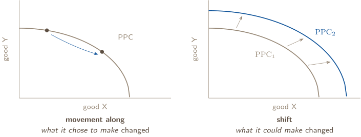
Movement along = the producer reallocated resources it already had. Cause: a change of plan, or a change in what is wanted. The curve does not move, and the move has a real opportunity cost — you can see it, because the point slides down one axis as it slides up the other.
Shift = the producer’s capacity itself changed. Causes worth naming: more or better resources (a bigger workforce, new machines, newly discovered land), improved technology or productivity, or — in the other direction — a disaster, a war, or a workforce leaving. Outward is economic growth; inward is contraction.
A move from inside the curve to the curve is not growth. Idle welders going back to work, or a misallocated crew reassigned, takes the producer from a point like B to a point on the frontier. Output rises, and nothing about capacity changed: the curve is where it was. The exam likes this one in a sentence — “the economy moved from inside its PPC to a point on it” describes falling unemployment or better allocation, and the correct label is a move toward efficiency, never economic growth. Growth is the curve itself moving out.
The shift that only moves one axis. If the improvement helps only one good — a new alloy usable in bike frames but useless for trailers — then that good’s intercept moves out and the other one does not. The curve pivots. A full outward shift would incorrectly claim that both capacities rose. Ask: could the producer now make more of the good on the other axis than before? If the honest answer is no, that intercept must not move.
CHECK 2 — READ THE CONSTRAINT
No. What improved is the use of the resources, not the stock of them: the economy was inside the curve wasting capacity and is now on it. Nothing about the frontier changed, so nothing about growth has been shown. Growth is the curve itself moving outward, and it needs more resources, better technology or more capital. One point moving is recovery; the whole line moving is growth, and on a graph the two look nothing alike.
THE GRAPH AS AN ANSWER FORMAT
When a free-response question says draw a correctly labeled graph, the requested relationships belong in the drawing itself. The College Board’s exam description puts graphing tasks at 30–50% of the free-response points. Use this as a completeness checklist; the exact prompt and scoring guideline decide how an individual response is evaluated.
1. | Label both axes with the goods, and with units if the question gave them. “Quantity” is ambiguous where “trail bikes per week” identifies both the good and period. |
|---|---|
2. | Name every curve. for the original, for the new one. An unnamed second curve cannot be read as a change. |
3. | Show the change with a direction. Draw the new curve and add an arrow from old to new. If only one intercept moves, only one intercept moves. |
4. | Mark and label any point the question refers to, and drop dashed lines to both axes if a value is being read off. |
5. | Answer any separate explanation request. If the prompt also says explain, write the causal statement it asks for: “The PPC shifts outward along the bike axis only, so the maximum number of bikes rises while the maximum number of trailers is unchanged.” A sentence is not automatically a separate requirement when the prompt asks only for a visual. |
Draw it large enough that every curve, point, and direction is unambiguous.
ABSOLUTE ADVANTAGE VS. COMPARATIVE ADVANTAGE
Absolute advantage — who can produce more of a good with the same resources (or produce one unit of it using fewer resources). It is a comparison of productivity, one good at a time, between producers.
Comparative advantage — who gives up less to produce it. It is a comparison of opportunity costs. This is the one that decides who should specialize in what, and it is the only one that determines the pattern of trade.
Read those two definitions again and notice they are not about the same thing. Absolute advantage compares output. Comparative advantage compares what was surrendered. A producer can be better at making everything and still should not make everything, because its time spent on one good is time not spent on the other, and that forgone output is the real cost.
The rule, in one line:
THE RULE
Compare opportunity costs, never outputs. The producer with the lower opportunity cost for a good has the comparative advantage in it and should specialize in it.
Two structural facts that let you check your answer.
When their opportunity costs differ, each producer has a comparative advantage in exactly one good in a two-producer, two-good problem. This follows from the reciprocal relationship: if my opportunity cost of drones is lower than yours, my opportunity cost of sensors — which is its reciprocal — must be higher than yours. So if your work says one producer has the comparative advantage in both goods, you have made an arithmetic error. Go back.
The boundary case: if the two producers have identical opportunity costs, neither has a comparative advantage in anything, and there are no gains from trade — there is no rate of exchange that beats what each could do at home. Trade is driven by differences in opportunity cost, not by differences in ability. The exam does occasionally hand you a table with equal ratios, and the correct answer is that no mutually beneficial trade exists.
Absolute advantage, by contrast, can be held by one producer in both goods, in one, or split. It carries no implication for who should trade with whom.
OUTPUT TABLES AND INPUT TABLES: THE SAME QUESTION, OPPOSITE ARITHMETIC
Both table types describe the same underlying technology. Which one you were handed decides which way your ratio runs, and reading the wrong way is the single most common source of a wrong comparative-advantage answer.
Output table — “per worker-day, Vantia makes 24 sensors or 12 drones.” Fix the resource, compare the goods.
The other good’s output goes on top. If it helps to have a phrase: other over own.
Input table — “a cabinet takes 8 labor-hours, a stool takes 2.” Fix the good, compare the resource each consumes.
Now the own good’s input goes on top — own over other, exactly reversed.
You do not have to memorize which is which. Both lines above are the same units chain, and if you build the chain the units settle it for you:
Labor-hours cancel; stools per cabinet survives. Set the second fraction up so the resource cancels, and there is only one way the numbers can go. Problems 4 and 5 are the same question in both formats, worked at the same slow pace.
Also worth knowing: you can convert one table into the other by picking any convenient amount of the resource and dividing. If a cabinet takes 8 labor-hours and a stool 2, then in 120 labor-hours the shop makes cabinets or stools — and running the output method on those gives stools per cabinet, the same answer. Converting and re-deriving is a genuine check, and Problem 5 uses it as one.
The third format: two PPC graphs. The exam often hands you no table at all — just each producer’s straight-line PPC with its intercepts. An intercept is an output table in disguise: it says how much of one good the producer makes when it makes nothing else. So the opportunity cost of the good on the horizontal axis is simply
and the comparative advantage in goes to the flatter curve.
These are Problem 6’s two countries over ten worker-days. Read the intercepts, divide, and the table you would have built from them is already done: Vantia’s drone costs 2 sensors, Solmar’s costs 4, so Vantia’s flatter curve carries the comparative advantage in drones. The reciprocal check still applies — the cost of a sensor is the horizontal intercept over the vertical one.
TERMS OF TRADE: THE RANGE WHERE A DEAL IS POSSIBLE
Autarky means no trade — each producer consumes only what it makes itself. Terms of trade is the exchange rate two producers agree on: how many sensors change hands per drone.
Nobody trades to be worse off, so each side has a walk-away number, and both walk-away numbers are opportunity costs the producer already knows:
the exporter of drones | will not accept less than it costs to make a drone at home. Its home cost is the floor. |
|---|---|
the importer of drones | will not pay more than it costs to make a drone at home — it would just make its own. Its home cost is the ceiling. |
For the strict-mutual-gain range — meaning both sides must be made strictly better off — use open bounds:
The floor is the lower of the two opportunity costs, and that producer — by definition — is the one with the comparative advantage. So the range is simply between the two producers’ opportunity costs for that good, and it is never empty unless the two are equal.
Why the strict range excludes the endpoints. At exactly the floor, the exporter receives precisely what making the drone cost it: it gains nothing and is indifferent. At exactly the ceiling, the importer pays precisely what making its own would have cost: same story for that side. But the other party still gains whenever the two home costs differ. An endpoint is therefore weakly beneficial — one indifferent, one strictly better off — not a zero-gain deal overall. If “mutually beneficial” means both must gain strictly, use the open interval. If the question permits one side to be indifferent, include the endpoints. Outside the closed interval, one side is worse off and will refuse.
Stating the range the other way round. A range of 2 to 4 sensors per drone is the same range as to drones per sensor — reciprocals, and the inequality flips end for end. Both are correct; just say which good you are pricing, and check that your two versions are reciprocals of each other before you write either down.
Gains from trade. When each producer specializes according to comparative advantage and then trades inside the range, both can consume a bundle outside their own PPC. That is the payoff of the whole topic, and it is worth being clear about what it does and does not say: their production possibilities have not changed at all — neither curve moved — but their consumption possibilities have. Specialization and exchange do not make anyone more capable; they stop capable resources being spent on the wrong things.
Complete or partial? With a straight-line PPC — as in the two-country trade examples below — opportunity cost is constant, so a producer with the comparative advantage keeps it at every quantity and specializes completely. On a bowed curve the cost rises as it specializes, and it stops where its cost climbs to the trading partner’s: specialization is partial. The exam works with the straight case; know that the bowed case exists so a prompt that mentions increasing costs does not read as a contradiction.
3. IGNORE WHAT CANNOT CHANGE
You have already paid a nonrefundable entry fee. One more activity gives $8 of benefit and costs $5. Should the entry fee affect this decision?
MARGINAL ANALYSIS: CHOOSE AN INCREMENTAL QUANTITY ONE UNIT AT A TIME
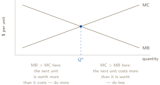
Marginal means from one more unit. Marginal benefit (MB) is the extra benefit the next unit brings; marginal cost (MC) is the extra cost that same unit adds. Both are differences between consecutive totals:
For a consumer, total benefit is measured as utility; for a firm, as total revenue — the two metrics the Course and Exam Description names, and the reason a consumer problem counts utils while a firm problem counts dollars.
Marginal cost is opportunity cost. It is what the resources consumed by that one extra unit would have produced elsewhere. This is not a separate idea bolted onto the unit — it is the same idea, applied one unit at a time.
The decision rule. Do the next unit whenever ; stop at the last unit for which that holds. For a smooth interior choice, the optimum sits where ; a boundary or discrete choice may require an inequality or adjacent tied quantities instead.

Why maximizes net benefit, rather than being a rule to memorize: every unit to the left of adds more benefit than cost, so skipping it leaves money on the table; every unit to the right adds more cost than benefit, so taking it destroys value. The total net benefit therefore climbs until MB and MC meet and falls afterwards, and the peak is where they cross. Problem 7 shows this on real numbers, with the total columns beside the marginal ones.
In a discrete table MB and MC may never be exactly equal. Then the rule is the one stated above: take every unit with and stop before the first unit where . If a unit lands exactly on , it adds precisely zero net benefit — taking it or leaving it gives the same total. Both adjacent quantities maximize net benefit; by convention a response may report the larger quantity where the equality occurs, provided the tie is acknowledged.
Sunk costs. A sunk cost is money already spent that no present decision can recover. It is not part of any marginal cost, so it cannot move the optimum — it subtracts the same constant from net benefit at every quantity. A sunk cost can make you regret starting; it can never tell you to stop at a different place.
CHECK 3 — IGNORE WHAT CANNOT CHANGE
No, and you do the activity: $8 of benefit against $5 of cost is worth $3, whatever the fee was. The fee is sunk — it is the same number whether you go on or stop, so it cannot differ between the two options, and only differences decide. The instinct to “get your money’s worth” is the trap this card exists for. Notice that the fee still matters for one question: whether to have bought the ticket at all. It just does not matter now.
TOTAL, MARGINAL, AND AVERAGE — THREE QUESTIONS, THREE ANSWERS
These get mixed up constantly, and each one answers a question the other two do not.
total | “Is this worth doing at all?” Compare total benefit with the avoidable total cost of each alternative still available. If doing none avoids all stated costs and TB TC at every positive quantity, choose none. An unavoidable sunk cost belongs to every current alternative, including zero output, so remove it before comparing them. |
|---|---|
marginal | “How much of it should I do?” Compare MB with MC and stop where they meet. This is the incremental method for locating the optimum; equivalently, compare total net benefit across feasible quantities. |
average | “What did a typical unit cost or deliver?” A summary of what has already happened. It cannot choose a quantity, because an average blends the units you should have done with the ones you should not have, and hides both inside one number. |
The average is the dangerous one, because comparing average benefit with average cost feels like a legitimate test and will often say “yes, keep going” well past the point where the extra units are destroying value. Problem 7(b) puts a number on what that mistake costs.
CONSUMER CHOICE: UTILITY, DIMINISHING RETURNS, AND THE LAST DOLLAR
Utility is satisfaction, counted in made-up units called utils. The units are arbitrary and only comparisons matter. Marginal utility (MU) is the extra utility from one more unit of a good.
The law of diminishing marginal utility: as you consume more of a good within a given period, each additional unit adds less utility than the one before. The third coffee of the day is genuinely worth less to you than the first. This is why MU columns fall as you read down them. It can support an interior answer — some of both goods — but does not rule out a corner where the consumer buys only one good.
The problem a consumer is actually solving. A budget is scarce resources, so this is an opportunity cost problem like every other one in the unit: a dollar spent on one good is a dollar unavailable for the other. The right comparison is therefore not which good gives more utility, but which gives more utility per dollar:
Divisible goods, an interior solution. When units can be divided, the consumer buys positive amounts of both goods, and more consumption still adds utility, total utility is maximized where the last dollar spent on each good gives the same marginal utility and the budget binds:
These are interior, divisible-good conditions, not a universal test. At a divisible corner, exact equality may be impossible: the last dollar on the chosen good gives at least as much utility as the first dollar that could be moved to the unchosen good. Under nonsatiation the budget still binds, but the comparison is an inequality.
Indivisible goods. Burritos and coffees arrive in whole units. The consumer must choose the highest-utility feasible bundle. The budget may have unusable money left, exact equality may never occur, and buying the currently highest ratio greedily need not find the best combination. Ratios remain useful evidence, but the decisive check is that no affordable addition or reallocation raises total utility — or, for a small table, that the best feasible bundles have been compared.
For a compact counterexample, suppose the budget is $4. Good X costs $3 and gives 6 utils, or 2 utils per dollar. Two units of Y cost $2 each and give 3.9 and 3.8 utils, ratios of 1.95 and 1.9. A greedy ratio rule chooses X and strands $1 for 6 utils; two Y units give 7.7 utils. Lumpy prices make the whole bundle, not the first ratio, decisive.
Why not just buy the good with the higher MU? Because that ignores what the good costs, and a dollar is the thing you are actually allocating. A $5 item delivering 50 utils gives 10 utils per dollar; a $3 item delivering 36 utils gives 12. The second has the lower marginal utility and is the better return per dollar. Problem 8 then verifies the final discrete bundle against the relevant feasible alternatives.
A scope note, so you do not waste study time: the College Board’s Course and Exam Description explicitly excludes indifference curves from AP Microeconomics. Comparing or equating marginal utility per dollar is in scope; the distinction among interior, corner, and whole-unit choices is part of using that comparison correctly.
PROBLEM 1
The cost that never appears on the receipt
Deven has a standing offer to work a 9-hour Saturday shift at a bakery for $16 per hour. He also has an open offer to tutor for $12 per hour for the same nine hours on those Saturdays. He takes neither, and instead runs a mobile bike-repair table. On a typical Saturday he collects $214 in repair fees, spends $63 on parts, and pays an $18 stall permit.
(a) What is his accounting profit for the Saturday? (b) What is the opportunity cost of spending the Saturday at the repair table? (c) What is his economic profit, and what does it say about the choice? (d) What would he have to collect in fees to be exactly indifferent between the table and his next-best option?
BEFORE YOU COMPUTE
The Unit 1 task is to identify and value the next-best alternative, including the implicit cost of Deven’s own time. The accounting-profit and economic-profit labels are a short preview of Topic 3.4; they are included here because their difference exposes the opportunity cost that a receipt omits.
The word doing the work in this prompt is instead. It tells you a resource — Deven’s Saturday — was used up, and that no receipt anywhere will record it.
So before any arithmetic, sort the three dollar amounts by whether money actually left his hands. Parts and the permit did; his time did not, and his time is the expensive part. That sort is the entire problem, and it is why an accountant and an economist will give different answers here without either of them making a mistake.
One trap is already visible in the prompt: he was offered two alternatives. Decide now which one belongs in the calculation, and be ready to say why the other does not.
WORKING
(a) Accounting profit. Take only the costs that left his hands — the explicit costs.
(b) Opportunity cost. The definition: the value of the next-best alternative forgone. Price both alternatives, in the same units, over the same 9 hours.
The hours cancel against “per hour” and what is left is dollars — which is what an opportunity cost measured against a wage should be.
Now choose. The bakery pays more, so the bakery is the next-best alternative, and the opportunity cost of the Saturday is $144.
It is not $144 + $108 = $252. He could not have worked the bakery shift and tutored in the same nine hours; taking one would already have cost him the other. Only one alternative was truly available to give up, and adding them counts the same Saturday twice. Whenever a prompt hands you three or more mutually exclusive uses of the same resource, compare them and keep the single most valuable forgone option.
(c) Economic profit. Economic cost counts both kinds:
Read that alongside part (a) and notice they are both true. He clears $133 in cash and is $11 per Saturday worse off than if he had taken the bakery shift. Negative economic profit does not mean the venture loses money; it means the resources in it — here, his Saturdays — would have paid more somewhere else.

The top bar is what came in; the bottom bar is what the Saturday truly cost, and it is longer. The pale $81 segment is the explicit cost an accountant records. The gray $133 plus the blue $11 together are the full $144 implicit cost an economist also charges; blue isolates the part revenue does not cover.
(d) The indifference point. Set economic profit to zero and solve for the fees he would need:
He collects $214, so he is $11 short — which is exactly the economic loss from part (c), as it must be. That agreement is the check: if your break-even figure and your economic profit do not reconcile to the same number, one of them is wrong.
At $225 in fees he is genuinely indifferent: the table and the bakery would leave him equally well off, and an economist would say the table is earning zero economic profit — covering every cost including the value of his time, and beating the alternative by nothing.
ANSWER
(a) $133 per Saturday (b) $144 — the bakery shift, the next-best alternative, and only that one (c) per Saturday; the table is profitable in cash and still not worth doing, because his Saturdays would earn $11 more at the bakery (d) $225 in fees
WATCH OUT
Two errors, each producing a specific wrong number.
Stopping at accounting profit gives $133 and the confident conclusion “yes, keep doing it.” That is the whole point of the problem and the reason implicit costs are examinable: the cash number is real and it recommends the wrong action.
Adding every alternative gives an opportunity cost of $252 and an economic profit of . Directionally it agrees with the right answer, which is what makes it dangerous — the conclusion looks fine and the number is wrong by $108. Next-best means next-best.
Charging a cost he would pay either way. Suppose Deven also pays $40 a week to park his van, table or no table. It is a real expense and it is not a cost of choosing the table, because the bakery Saturday would not have saved it. The opportunity cost of a choice counts only what that choice changes — the exam’s version is the student who lists room and board as a cost of attending college, when they would eat and sleep somewhere either way.
CONNECTION
Most quantitative problems that follow repeat this comparison with the units changed. Here the thing given up was a wage, in dollars. On a production possibilities curve it will be trailers given up per bike gained; in a trade problem, sensors given up per drone; in Problem 7, whatever the resources spent on one more storm-drain filter would otherwise have produced. Same question, different units: what did you give up?
ABOUT THIS EXCERPT
This is the opening of a 66-page guide: the diagnostic tree, the full Master Toolbox, and the first worked problem. 8 more problems follow in the complete guide, each worked the same way — what to notice before you start, every step shown, and the mistake that problem invites. The complete guide is shared with families during the fit conversation.
Engineering Confidence — engineeringconfidence.one
Source and review notes
What this resource is
Complete browser edition of the public excerpt from an original Engineering Confidence AP Microeconomics packet aligned to the College Board framework effective Fall 2026. All problems are original.
- Published
- Last reviewed
- Printable edition
- 27 pages
Course reference: official College Board course page.
Read this public excerpt above, or save the PDF for printing and offline reading.
Download the 27-page PDF excerpt