Read the public excerpt
The same instruction and worked examples appear here and in the printable PDF excerpt. You can request full guides for upcoming units below.
READ THIS FIRST
About this guide. Unit 2 drew a market. Unit 3 opens the door of one of the firms inside it and asks the question every producer answers every day: how much should I make? The answer is the same at every step of the unit — one more unit is worth making when what it brings in covers what it costs to make — and the whole of the unit is the machinery for saying what that costs. Workers produce output, the production function says how much; output costs money, the cost curves say how much per unit; a price arrives from the market, and the firm compares it with the cost of the next unit. Everything else — shutting down, leaving the industry, the long run, efficiency — is that comparison made at a different moment.
The College Board calls this unit “not always intuitive” and says so in its own note: students benefit from “multiple opportunities to practice drawing and interpreting graphs that represent perfect competition,” and “questions on the AP Exam that cover long-run production costs are often challenging.” With Unit 2 it carries the heaviest weight in the course — 22 to 25 percent of the multiple-choice section — and its cost curves are the ones every market structure in Unit 4 is drawn on top of.
The graph is the answer format. A free-response question in this unit hands you a price and asks for a firm’s output, profit or loss, and whether it should operate — and it scores the graph: the marginal cost curve, the average cost curves, the horizontal price line, the quantity where marginal revenue meets marginal cost, and the rectangle between price and average total cost. Every figure here is drawn the way a scored response has to be drawn, so the picture you copy into your own work is already a picture that scores.
One firm runs through the guide. Its production table appears in Problem 1, its costs in Problem 2, and the same numbers return in Problems 5, 6 and 7, so that by the end you have seen one business decide everything a business decides. A four-function calculator is permitted on both sections of the exam; every number here is carried at full precision and rounded once.
Every topic in the unit, and where it lives. The College Board lists seven; here is each one and the page that teaches it.
- 3.1 the production function — card 1 (p. 14); Problem 1.
- 3.2 short-run production costs — card 2 (p. 16); Problem 2.
- 3.3 long-run production costs — card 3 (p. 18); Problem 3.
- 3.4 types of profit — card 4 (p. 19); Problem 4.
- 3.5 profit maximization — card 5 (p. 21); Problem 5.
- 3.6 firms’ short-run decisions to produce and long-run decisions to enter or exit — card 6 (p. 23); Problem 6.
- 3.7 perfect competition — card 7 (p. 25); Problem 7.
Card 8 (p. 26) is the side-by-side graph — what a scored perfect-competition diagram has on it, in the order the scorer looks.
WHERE THE POINTS GO ON THIS UNIT
The College Board’s own note on this unit names two places: the graphs of perfect competition, which students should practice “drawing and interpreting” until they can, and long-run production costs, which are “often challenging” — though, the note adds, they do not “comprise a significant portion of the AP Exam.” Graphing is 30 to 50 percent of every free-response point in this course, and the firm’s graph is the one drawn most. In 2026, 68% of the cohort earned a 3 or higher; on the last worksheet the College Board released for this exam, in 2012, a 5 began at 78.9% of the composite score — there is little room to lose graph points and still reach the top.
Marginal, not average, decides output. On a smooth rising MC curve, compare marginal revenue with marginal cost. For a table with indivisible batches or initially falling MC, compare profit at every feasible output, including zero. The average curves say what profit is once output is chosen; they never say what output to choose. Choosing output at minimum average total cost is the named error of this unit, and it produces the wrong quantity almost every time.
Profit is a rectangle, and it has two corners you must find. Height: price minus average total cost, read at the profit-maximizing quantity — not at the minimum of the curve. Width: that quantity. A response that shades the right area but cannot say why it is that area earns the drawing points and loses the reading points; say it, then shade it.
Two runs, two decisions. Shutting down is a short-run choice made against average variable cost: keep producing if price covers it. Exiting is a long-run choice made against average total cost: leave if price cannot cover it once every cost is variable. A firm can be losing money and correctly stay open; the exam asks which decision, and which curve, in the same breath.
The formula is part of the answer. Write , then the numbers, then the result with its unit — dollars per unit. A bare number earns the number’s point and nothing for the method the question was written to test.
Diagnostic Decision Tree
How to use it. The pages that follow are your concept reference: a diagnostic decision tree, a symptom map, then a Master Toolbox of eight cards — seven for the seven College Board topics, in order, and one for the graph itself — carrying every definition, every formula and every figure the seven problems use. Use the tree when you are starting a problem; use the map when you are stuck inside one; open the card you need rather than reading them all. Then, for each problem: read the prompt, read the “Before you compute” rail, and attempt the problem yourself before reading the worked solution. If it is late, at minimum cover the “Working” section and predict its first line.
READ WHAT YOU WERE HANDED, BEFORE YOU READ THE QUESTION
Unit 3 has seven routes, and the prompt signals one before it asks anything — in the shape of the data or the situation it hands you. Sort on that first.
1. A table of workers and output. Production: compute marginal product from the differences and average product from the ratios, find where marginal product turns down, and say why. Card 1, Problem 1.
2. A cost table, or cost curves. Costs: fixed apart from variable, marginal from the change in total, averages from the totals. Card 2, Problem 2. If the question is about a change in wages or rent, ask which curves that cost lives in.
3. Plant sizes, or “in the long run.” Long-run costs: every input variable, the envelope of short-run average costs, economies and diseconomies of scale, the minimum efficient scale. Card 3, Problem 3.
4. Revenues and costs with an owner in the story. Profit types: explicit costs make accounting profit; add the implicit costs and you have economic profit, and only economic profit drives the decision. Card 4, Problem 4.
5. A price, and “how much should the firm produce.” Profit maximization: marginal revenue equals marginal cost; for a price taker, marginal revenue is the price. Then profit as the rectangle. Card 5, Problem 5.
6. A price below average total cost. The two decisions: compare price with average variable cost for the short run, with average total cost for the long run. Card 6, Problem 6.
7. A market beside a firm, or “what happens in the long run.” Perfect competition: the firm takes the market’s price, profits invite entry, entry shifts market supply, price falls to minimum average total cost, and economic profit goes to zero. Card 7, Problem 7 — and card 8 before you draw.
Where to Look When You’re Stuck
HOW TO USE THIS MAP
The tree above is for a problem you are about to start. This table is for one you are already inside. Find your sentence, do the move in the middle column, then turn to the card or problem on the right.
PRODUCTION, COSTS AND PROFIT
What is happening | First move | Where |
|---|---|---|
“Where do diminishing returns start?” | Compute marginal product for each worker; it is the first worker whose marginal product is smaller than the one before. | p. 14, Prob. 1 |
“My marginal cost numbers don’t match the key” | Marginal cost is the change in total cost over the change in output, not per worker. With a wage, . | p. 16, Prob. 2 |
“Which curves move when rent goes up?” | Rent is fixed: AFC and ATC rise; MC and AVC do not move. A wage rise moves MC, AVC and ATC. | p. 16, Prob. 2 |
“Economies of scale or diminishing returns?” | Returns are short run, one input varying; scale is long run, every input varying. Different curves, different words. | p. 18, Prob. 3 |
“The firm makes money and the key says it should leave” | Accounting profit ignores implicit costs. Subtract the owner’s forgone salary and interest; if the result is negative, economic loss. | p. 19, Prob. 4 |
OUTPUT, SHUTDOWN AND THE LONG RUN
What is happening | First move | Where |
|---|---|---|
“How much should it produce?” | Compare total profit at feasible outputs, including zero. Use the rising MC branch for a smooth model; minimum ATC alone does not choose output. | p. 21, Prob. 5 |
“Which rectangle is the profit?” | Height at the chosen quantity; width that quantity. Name it, then shade it. | p. 21, Prob. 5 |
“It’s losing money — shut down?” | Compare price with average variable cost. Above it, operate; the loss is smaller than the fixed cost. Below it, shut down. | p. 23, Prob. 6 |
“Shut down or exit?” | Shutdown is short run (price against AVC); exit is long run (price against ATC, when every cost is variable). | p. 23, Prob. 6 |
“Why does the price fall in the long run?” | Profit invites entry; entry shifts market supply right; price falls until economic profit is zero at minimum ATC. | p. 25, Prob. 7 |
“Allocative or productive?” | Allocative: . Productive: production at minimum ATC. Long-run perfect competition has both. | p. 25, Prob. 7 |
“My graph is right and I still lost points” | Run card 8. Both axes, every curve named, the price line, the quantity at MR MC, the rectangle’s two corners. | p. 26, Prob. 5, 7 |
If none of those is your sentence, the final section of this guide is the longer version. It is organized by what went wrong, not by the vocabulary term you were supposed to remember.
Master Toolbox — Everything These Problems Use
Eight cards. Each one is a definition, the mechanism behind it in plain words, and the figure that carries it. The firm in the figures is the firm in the problems: a fixed cost of $60, a wage of $20 per worker, and the production table of Problem 1.
1. THE PRODUCTION FUNCTION: TOTAL, MARGINAL, AVERAGE — AND THE TURN
The production function relates inputs to output. In the short run at least one input — the plant, the ovens, the land — is fixed, and the firm changes output by changing the variable input, usually labor. Three numbers describe what each worker does:
Diminishing marginal returns. As more of the variable input is added to a fixed input, the marginal product eventually falls: the fourth worker has less of the fixed oven to work with than the third did. Marginal product can rise at first — specialization, the division of labor — but the fixed input always wins in the end. The CED’s definition is exactly that sentence: diminishing marginal returns “occur as the firm employs more of one input, holding other inputs constant.”
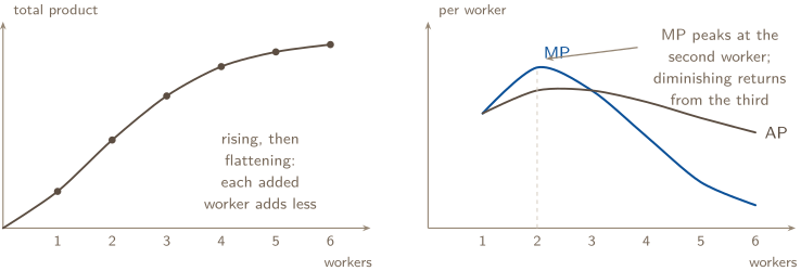
The two readings that score. Diminishing marginal returns begin with the first worker whose marginal product is lower than the previous worker’s — here the third. And average product rises while marginal product is above it and falls once marginal product drops below it, so the two cross where average product peaks. The average is pulled toward the marginal, always; that is arithmetic, not economics, and it returns in card 2 as the reason marginal cost cuts the average cost curves at their minimums.
A check first. One question opens three of the cards below and is answered at that card’s end. Answer it before you read on. Getting it wrong is the point — that is what makes the card stick.
1. CHANGE ONE COST
Rent rises while wages and the production technology stay fixed. Which curves move: MC, AVC, ATC?
2. SHORT-RUN COSTS: SEVEN NUMBERS FROM TWO, AND THE SHAPE THEY MAKE
In the short run a firm pays for the fixed input whether it produces or not — total fixed cost, TFC, constant at every output including zero — and pays for the variable input in proportion to how much it uses — total variable cost, TVC. Everything else is a ratio or a difference:
Why marginal cost is U-shaped. With a wage per worker, the cost of one more unit is the wage divided by how many units the next worker adds: . When marginal product rises, marginal cost falls; when diminishing returns set in and marginal product falls, marginal cost rises. The CED states the link directly: “production functions with diminishing marginal returns yield an upward-sloping marginal cost curve.”
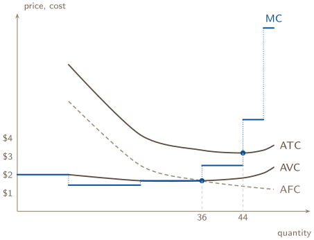
Table or smooth model? Ferris can choose the whole-worker outputs in its table. Its batch MC need not equal price at the best output; compare total profit at every feasible output, including zero. In a smooth model, an interior optimum on rising MC satisfies MR MC. The familiar MC-at-minimum-average relationships describe that smooth model; the table shows their discrete counterpart. AVC is minimized at both 24 and 36 here; ATC is minimized at 44.
The three shapes to know by sight. AFC falls forever — the same fixed cost spread over more units. AVC and ATC are U-shaped, and ATC sits above AVC by exactly AFC, so the gap closes as output grows. MC crosses each average curve at its minimum: while the marginal unit costs less than the average, it pulls the average down; once it costs more, it pulls the average up. What shifts them: a change in the wage or in productivity moves MC, AVC and ATC; a change in rent or another fixed cost moves AFC and ATC and leaves MC and AVC alone. Specialization and the division of labor lower marginal cost.
CHECK 1 — CHANGE ONE COST
ATC only. Rent is a fixed cost: it does not change with output, so it cannot change the cost of one more unit — MC is untouched — and it is not a variable cost, so AVC is untouched too. It raises AFC at every quantity, and ATC is AVC plus AFC, so ATC rises and its minimum shifts right. The test is always the same: ask whether the cost changes when output changes. A cost that does not vary cannot move a marginal or a variable curve.
3. LONG-RUN COSTS: EVERY INPUT VARIABLE, AND WHAT SCALE DOES
In the long run “firms can adjust all their inputs, and as a result, all costs become variable.” There is no fixed cost, no AFC, and no diminishing returns in the short-run sense — the firm chooses its plant size along with its labor. The long-run average total cost curve, LRATC, traces the lowest average cost of each output when the plant is chosen freely: the envelope of every short-run ATC curve.
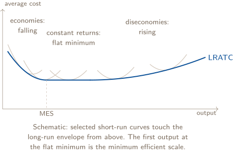
The vocabulary, and what each word measures. Returns to scale describe output when all inputs change together: doubling every input more than doubles output (increasing), doubles it (constant), or less than doubles it (decreasing). Economies of scale describe the LRATC curve: falling as output grows (economies — bulk buying, specialization, spreading design costs), flat (constant returns, the efficient scale), rising (diseconomies — coordination and management strain). The minimum efficient scale, MES, is the smallest output at which LRATC reaches its minimum.
Why the exam cares. MES against the size of the market decides how many firms can fit: an MES that is a large share of market demand leaves room for a few large firms; an MES that is tiny beside the market leaves room for many, which is the perfect competition of card 7. Diminishing returns and diseconomies of scale are different things — one input against a fixed one in the short run, every input together in the long run — and mixing the words is the loss the CED’s note anticipates.
4. TYPES OF PROFIT: THE COST THE ACCOUNTANT DOES NOT SEE
Explicit costs are paid out — wages, rent, materials, interest on a loan. Implicit costs are what the owner’s own resources could have earned elsewhere — the salary given up to run the business, the interest the invested savings would have paid, the return that compensates for risk. Two profits follow:
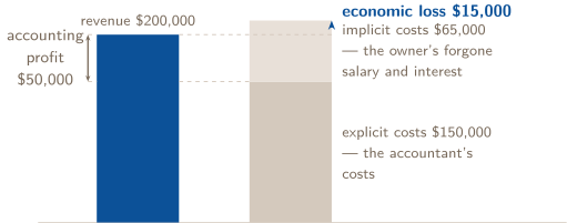
Which one decides. “Firms respond to economic profit (loss) rather than accounting profit.” An owner earning a $50,000 accounting profit who could earn $65,000 by closing and taking a job is losing $15,000 a year by staying, and in the long run leaves. Normal profit is the accounting profit that just covers the implicit costs — the return the owner needs to stay — and it corresponds to zero economic profit. When card 7 says firms earn zero economic profit in long-run equilibrium, it means they earn exactly a normal profit: enough to stay, not enough to attract anyone else.
2. CHECK THE SHORTCUT
In a table, marginal cost first falls and then rises, and the first batch costs more than the market price. Is that enough to stop, without looking at any later output?
5. PROFIT MAXIMIZATION: THE MARGINAL RULE, AND THE RECTANGLE IT PRODUCES
A firm chooses the feasible output with the highest total profit, including zero output. With smooth curves, an interior optimum on rising MC satisfies MR MC, subject to the shutdown comparison. With Ferris’s table, evaluate each complete output choice: early batches cannot be skipped just because a later batch has lower marginal cost. A falling-then-rising MC schedule makes “stop at the first expensive batch” an unsafe shortcut.
Marginal revenue for a price taker. A perfectly competitive firm sells every unit at the market price, so each unit adds exactly to revenue: , a horizontal line at the market price, which is also the demand curve the firm faces. The rule becomes .
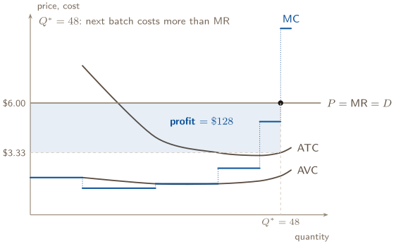
Profit as an area. Once is chosen, profit per unit is read at , and total profit is that height times : the rectangle between the price line and the ATC curve, from the axis to . Equivalently . Both give the same number, and the exam accepts either — but the rectangle’s height is ATC at the chosen quantity, never at the curve’s minimum. When price is below ATC the same rectangle is a loss.
CHECK 2 — CHECK THE SHORTCUT
No. “Stop at the first unit whose cost exceeds the price” is a rule for a rising marginal cost curve. While MC is still falling, an early batch can cost more than the price and a later one much less, so stopping at the first failure can leave the firm at zero when a positive output was profitable. On a table, compare total profit at every feasible output — including zero — and let the numbers choose. The marginal rule is a shortcut that is only valid on the rising branch.
3. SEPARATE THREE QUESTIONS
At its best positive output a price-taking firm has , and . Is it profitable? Should it shut down now?
6. PRODUCE OR SHUT DOWN; STAY OR EXIT — TWO RUNS, TWO CURVES
A firm can lose money and still be right to keep producing. The short-run question is whether producing loses less than not producing — and not producing still costs the fixed cost.
The shutdown rule. Compare total revenue with total variable cost at the best positive output. If there, operating covers variable cost and contributes toward fixed cost. If the firm makes a loss, that loss is smaller than TFC. If , operating loses more than shutting down, so choose zero output. At , operating and shutting down tie: both lose exactly TFC.
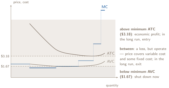
The long-run rule. Once every cost is variable there is no fixed cost to keep paying, and the comparison is price against average total cost. Economic losses — price below minimum ATC — lead firms to exit the market; economic profits lead firms to enter, if nothing bars them. So a price between minimum AVC and minimum ATC is a firm that operates today and leaves eventually. The exam asks “should the firm shut down” and “will firms exit” as different questions, and card 7 draws what the exits do to the price.
CHECK 3 — SEPARATE THREE QUESTIONS
No and no — and those are two different answers, not one. The firm is losing money, because $4 of revenue per unit against $5 of average total cost is a $1 loss on every unit. But it should keep producing in the short run, because $4 covers the $3 of variable cost with $1 left over toward the fixed cost it owes either way; shutting down would lose the whole fixed cost instead of part of it. Profitability and shutdown are decided by different curves — ATC for the first, AVC for the second — and the long-run exit question is a third.
7. PERFECT COMPETITION: THE PRICE TAKER, THE LONG RUN, AND WHY IT IS EFFICIENT
A perfectly competitive market has many buyers and sellers of an identical product, with no barriers to entry or exit and no market power: “firms can sell all their outputs at a constant price determined by the market.” The firm is a price taker. Its demand curve is horizontal at the market price, which is also its marginal revenue, and it chooses output where .
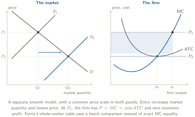
Short run to long run. At the firm earns economic profit (price above ATC). With no barriers, new firms enter, market supply shifts right, and the price falls; entry stops when the price reaches minimum average total cost, where the last firm to enter earns exactly zero economic profit — a normal profit, card 4. Losses run the film backward: exit, supply shifts left, price rises to the same point. In long-run equilibrium, and economic profit is zero.
Why that is efficient. Allocative efficiency: — the price the last buyer paid equals the cost of the last unit made, so the market produces exactly the units worth more to a buyer than they cost to make. Productive efficiency: every firm produces at minimum ATC, the lowest cost per unit its technology allows. Prices in a competitive market “communicate to consumers and producers the magnitude of others’ marginal costs of production and marginal benefits of consumption.” A perfectly competitive market in long-run equilibrium has both efficiencies; Unit 4’s structures each give one or both up.
Cost industries. Whether the long-run price returns to the old level depends on what entry does to costs. In a constant-cost industry input prices do not change with entry and the long-run supply curve is horizontal at minimum ATC. In an increasing-cost industry entry bids up input prices, ATC rises, and long-run supply slopes upward. In a decreasing-cost industry entry lowers input costs and long-run supply slopes downward. The long-run price “depends on the portion of the long-run cost curves on which firms operate.”
8. THE GRAPH THE EXAM SCORES
A correctly labeled perfect-competition diagram is a checklist, and the scorer runs it in this order. Draw in the same order and nothing is forgotten.
- 1.
- Two graphs, side by side, when the market is in the question: the market on the left with price and market quantity, the firm on the right with price, cost and quantity. The price line runs across from one to the other.
- 2.
- Every curve named: and on the market; MC, ATC, AVC on the firm; the horizontal line at the market price labeled (for the firm).
- 3.
- The quantity, dropped to the axis, at the point where MR crosses MC on MC’s rising side.
- 4.
- The rectangle, when profit or loss is asked: from the axis to , between the price line and ATC at . Say which it is — profit if price is above ATC, loss if below.
- 5.
- The shift, when the long run is asked: the new supply curve named and arrowed on the market, the new price line drawn across to the firm, and the new quantity dropped.
- 6.
- The words: which decision (produce or shut down; enter or exit) and which curve decided it.
Two habits that cost nothing. Write MC’s label at its top and the averages’ labels at their right ends, so no label sits on a crossing. And draw the price line first, then find from it — the order in which the firm itself decides.
The Problems — In Topic Order
Seven problems, one per topic, in the order the College Board lists them, all about one firm. Every number is original. Work each one before reading its solution.
PROBLEM 1
The production function: from a table of workers to the turn
Ferris Cabinetry builds a single model of cabinet in a workshop with a fixed set of tools. Its output per day, by number of workers:
| Workers | 0 | 1 | 2 | 3 | 4 | 5 | 6 |
|---|---|---|---|---|---|---|---|
| Cabinets per day | 0 | 10 | 24 | 36 | 44 | 48 | 50 |
(a) Compute the marginal product and the average product of each worker. (b) Identify the worker with whom diminishing marginal returns begin, and explain why they begin at all. (c) Identify where average product is highest and explain its relationship to marginal product there. (d) The workshop is the fixed input. Explain what would change about the table in the long run.
BEFORE YOU COMPUTE
Marginal product is a difference — this row’s output minus the last row’s. Average product is a ratio — output over workers. Write both formulas before the numbers; the CED’s task is “calculate,” and the formula is scored.
Diminishing returns begin at the first worker whose marginal product is lower than the previous worker’s — not at the first worker whose marginal product is small, and not where total product falls (it never does here).
WORKING
(a) and :
| Workers | 1 | 2 | 3 | 4 | 5 | 6 |
|---|---|---|---|---|---|---|
| Total product | 10 | 24 | 36 | 44 | 48 | 50 |
| Marginal product | 10 | 14 | 12 | 8 | 4 | 2 |
| Average product | 10.0 | 12.0 | 12.0 | 11.0 | 9.6 | 8.3 |
The second worker’s marginal product: cabinets. The fifth’s average product: cabinets per worker.
(b) Marginal product rises from 10 to 14 with the second worker and falls to 12 with the third: diminishing marginal returns begin with the third worker. They begin because the workshop and its tools are fixed. Two workers can divide the tasks and share the tools efficiently; a third adds output, but with less tool time and floor space per worker, so adds less than the second did. Each additional worker has less of the fixed input to work with, and the marginal product falls — the definition the CED gives, one input rising against the others held constant.
(c) Average product is highest — 12.0 — at two and three workers. The third worker’s marginal product is exactly 12, equal to the average, which is why the average neither rises nor falls: a marginal above the average pulls it up (the second worker, MP 14 against AP 10, lifted AP to 12); a marginal below the average pulls it down (the fourth, MP 8, drags AP to 11). Marginal product crosses average product at the maximum of average product. The same arithmetic returns in Problem 2 for costs.
(d) In the long run the workshop is no longer fixed: Ferris can build a bigger shop, buy more tools, or open a second site along with hiring. There is then no fixed input for the variable one to crowd, so the diminishing returns in the table — which come from adding workers to one shop — no longer apply. What replaces them is the question of scale in Problem 3: does doubling everything double output, or more, or less.
ANSWER
(a) MP: 10, 14, 12, 8, 4, 2; AP: 10.0, 12.0, 12.0, 11.0, 9.6, 8.3.
(b) The third worker — marginal product falls from 14 to 12, because the
fixed workshop gives each added worker less to work with.
(c) Two to three workers, AP ;
there MP
AP, and MP crosses AP at AP’s maximum.
(d) All inputs variable, so no fixed input to crowd; the table becomes a
question of returns to scale.
WATCH OUT
Reading diminishing returns off total product. Total product rises through the sixth worker. Diminishing returns are about the marginal product falling, not the total; the table shows both, and only one answers the question.
“Diminishing returns because workers get lazy.” The mechanism is the fixed input, not the workers. Same skill, less oven; that is the sentence.
CONNECTION
Divide the wage by each marginal product and you have the marginal cost of a cabinet, which is Problem 2’s whole table. The turn at the third worker in this problem is the turn in marginal cost there — diminishing returns are what make marginal cost rise, and everything from Problem 5 onward depends on marginal cost rising.
ABOUT THIS EXCERPT
This is the opening of a 34-page guide: the diagnostic tree, the full Master Toolbox, and the first worked problem. 6 more problems follow in the complete guide, each worked the same way — what to notice before you start, every step shown, and the mistake that problem invites. The complete guide is shared with families during the fit conversation.
Engineering Confidence — engineeringconfidence.one
Source and review notes
What this resource is
Complete browser edition of the public excerpt from an original Engineering Confidence AP Microeconomics packet aligned to the College Board framework effective Fall 2026. One original firm runs through every problem.
- Published
- Last reviewed
- Printable edition
- 16 pages
Course reference: official College Board course page.
Read this public excerpt above, or save the PDF for printing and offline reading.
Download the 16-page PDF excerpt