Read the public excerpt
The same instruction and worked examples appear here and in the printable PDF excerpt. You can request full guides for upcoming units below.
READ THIS FIRST
About this guide. Unit 1 is a third of the AP Precalculus exam — 30 to 40 percent — and it is built on two ideas the College Board names in its first sentence: covariation, how the output changes in tandem with the input, and rates of change, including the rate at a point and the way rates themselves change. Every polynomial and rational function in the unit is a vehicle for those two ideas, and the exam grades the sentences you write about them as much as the numbers: “on the interval from to , the average rate of change of is cubic meters per minute” is the CED’s own model of a full answer, with the function, the interval, the number and the units all in it.
Three mistakes to learn to catch:
- A rate without its interval, or its units. “The rate is 0.4” names nothing. Every rate in this unit is an average over a stated interval, or an approximation at a point from a small interval around it, and the sentence carries the interval, the units, and the sign.
- Concavity read from the height instead of from the rate. A graph that is rising can be concave down; concave up means the rate of change is increasing. The check is the rates over equal steps, not the picture’s slope.
- A hole called an asymptote, and a zero of the denominator called a zero of the function. Both are settled by multiplicities, and the factored form is where they show.
Every topic in the unit, and where it lives. The College Board lists fourteen; here is each one and the page that teaches it.
- 1.1 change in tandem: function, domain and range, increasing and decreasing, concavity, zeros — card 2 (p. 12); Problem 1.
- 1.2, 1.3 average rate of change, the rate at a point, and how rates change for linear and quadratic functions — card 3 (p. 14); Problems 1 and 2.
- 1.4 polynomials and their rates of change: extrema, inflection — card 4 (p. 15); Problem 3.
- 1.5 zeros, multiplicity, complex zeros, th differences, even and odd functions — card 5 (p. 16); Problems 2 and 3.
- 1.6, 1.7 end behavior of polynomials and of rational functions — cards 6 and 7 (p. 17); Problem 4.
- 1.8, 1.9, 1.10 zeros, vertical asymptotes and holes of rational functions — card 8 (p. 20); Problem 5.
- 1.11 equivalent representations, long division, the binomial theorem — card 9 (p. 21); Problem 6.
- 1.12 transformations — card 10 (p. 22); Problem 7.
- 1.13, 1.14 choosing a function model, its assumptions and restrictions, and building and applying it — cards 11 and 12 (p. 23); Problems 8 and 9.
How to use it. The decision tree, the symptom map and the Master Toolbox are reference, not assigned reading. Route the problem, open the matching card, and attempt the prompt before reading the worked solution. Part of the exam expects a graphing calculator — for zeros, intersections, extrema and regressions — and every place this guide reaches for one says so; everywhere else the work is by hand. What nine problems cannot do is give you enough repetitions; each is the clearest instance of its shape, so a problem you found easy is a signal to go find five more like it.
WHERE THE POINTS GO ON THIS UNIT
The first cohort to sit this exam, in 2024, had 75.6% score a 3 or higher — nearly double AP Physics 1’s debut on the same kind of first sitting — and the free-response section is where the difference between a 3 and a 5 is decided, because the College Board says in this unit’s own exam note that “students will not only be required to arrive at a solution but also explain and provide rationales for their conclusions.” Four places the rationale goes missing:
Every one of them is the same omission wearing a different hat: a result with no rationale tied to the representation it came from. Name the interval and the units for a rate; keep a domain restriction after you simplify; and say “the table suggests” when the table is all you have.
The precise sentence. The CED’s model: “On the closed interval 0 to 1, as the value of increases, the value of increases then decreases.” And for a rate: the function, the interval, the number, the units. Students “need to use clear language when referring to variables and functions, including units of measure.” A number with no interval and no unit is not a rate of change; it is a number.
The reason behind a limit statement. “” earns its point with the why: the quotient of leading terms is . “Vertical asymptote at ” earns it with the multiplicities: a zero of the denominator that the numerator does not cancel. The exam asks for the justification in words.
The calculator’s answer, then the sentence. “Part of the exam relies on technology,” and students “must learn to identify zeros, points of intersection, and extrema using graphing calculator technology” and “calculate linear, quadratic, cubic, and quartic regressions.” The point is not the button; it is reporting the value to three decimal places, naming what it is — a local maximum of at — and answering the question that was asked about it, in context.
The model’s assumptions and restrictions. Topic 1.13’s second objective is to describe assumptions and restrictions: a domain restriction from the context ( for a box cut from a 20-centimeter sheet), a range restriction from rounding, a stated assumption about what stays constant. A model presented without them is half a model, and the exam asks for the other half by name.
Diagnostic Decision Tree
HOW TO READ THE PROMPT
Run these in order, before touching a formula or a calculator. Each one rules out whole families of tools.
1. Is the question about how two quantities change together, or about a specific function’s features? “Describe how changes as increases” — change in tandem: increasing, decreasing, concavity, zeros, in the CED’s sentence. “Find the asymptotes of ” — features, and the factored form is the tool.
2. Is a rate of change asked for? Over an interval — the average rate, , a secant’s slope, with units. At a point — approximate it from average rates over small intervals containing the point, and say that you did. How the rate is changing — concavity, from average rates over equal steps: increasing rates, concave up.
3. Is it a polynomial? Read the degree and the leading coefficient for end behavior; the factored form for zeros and their multiplicities; the zeros for where local extrema must sit between them; even degree for a global maximum or minimum. Complex zeros come in conjugate pairs and never touch the graph.
4. Is it a rational function? Factor top and bottom. A zero of the numerator that is in the domain is a zero of the function. A zero of the denominator is a vertical asymptote or a hole, decided by comparing multiplicities. End behavior is the quotient of leading terms: a horizontal asymptote, , or a slant or polynomial asymptote from division.
5. Are two forms of the same function on the page? Factored reveals zeros, holes and asymptotes; standard reveals end behavior; division reveals the slant asymptote; the binomial theorem expands a power of a binomial. The exam asks which form answers which question.
6. Is a graph moved, stretched or reflected? up, left by , vertical dilation, horizontal dilation by ; negatives reflect. Track one point through every step, in order, and say what happened to the domain and range.
7. Is a model being chosen, built or applied? Choose from how the quantities vary, never from what they are called: a constant rate suggests linear, constant nonzero second differences at equal steps suggest a quadratic, inverse proportion suggests a rational model — and “area” or “volume” on its own settles nothing until you write how each dimension depends on the input. Build from the restrictions, from a transformed parent, or from a regression. Apply with units, and with the assumptions and the domain named.
Where to Look When You’re Stuck
FIND THE SENTENCE THAT SOUNDS LIKE YOUR SITUATION
The tree above is for a problem you are about to start. This table is for one you are already inside. Find your sentence, do the thing in the middle column, turn to the page on the right.
What is happening | First move | Where |
|---|---|---|
“It says describe and I wrote a number” | The CED’s sentence: on this interval, as increases, does what; concave which way; zeros where. | p. 12, Prob. 1 |
“Average rate, or the rate at a point?” | An interval in the words: the secant slope. A single moment: average rates over small intervals around it, and say “approximately.” | p. 14, Prob. 1 |
“Is it concave up or down?” | Rates over equal steps: increasing means concave up. Never the height. | p. 14, Prob. 2 |
“What degree is this table?” | Take differences until they are constant; the number of rounds is the degree. | p. 16, Prob. 2 |
“Does the graph cross or bounce at this zero?” | Odd multiplicity crosses; even multiplicity is tangent and bounces. | p. 16, Prob. 3 |
“Where does it go at the ends?” | Polynomial: the leading term. Rational: the quotient of leading terms. | p. 17, Prob. 4 |
“Asymptote or hole?” | Factor both. Denominator’s multiplicity larger: asymptote. Numerator’s at least as large: a hole, at the limit’s height. | p. 20, Prob. 5 |
“A slant asymptote” | Numerator one degree higher: divide, keep the quotient, drop the remainder. | p. 21, Prob. 6 |
“Which form do I want?” | Zeros and holes: factored. End behavior: standard. Slant: division. : the binomial theorem. | p. 21, Prob. 6 |
“Which way does move?” | Left. Inside the function, the sign is backwards; outside, it is not. Track one point. | p. 22, Prob. 7 |
“Which kind of model?” | Read how the quantities vary. Check rates or equal-step differences, then test a candidate model against the context. | p. 23, Prob. 8 |
“Build the model from what was given” | Zeros give factors; one more point gives the leading coefficient; the context gives the domain. | p. 24, Prob. 9 |
If none of those is your sentence, the last section of this guide is the longer version, organized by what went wrong.
Master Toolbox — Everything These Problems Use
Use these cards as you work. Name the decision you need to make, then open the relevant card. Each card stands on its own; you do not need to read the whole toolbox before attempting a problem.
1. THE SENTENCE THE EXAM GRADES, AND THE VERBS THAT ASK FOR IT
Describe | the CED’s sentence: On the interval from to , as increases, increases at a decreasing rate; name the function, the interval, the direction, the concavity. |
|---|---|
Calculate a rate | the quotient written, the number, the units — cubic meters per minute — and the interval it belongs to. |
Justify / explain | the mechanism: the leading term, the multiplicity, the differences that were constant, the quotient of leading terms. The claim alone is half the credit. |
Determine (with technology) | the value to three decimal places, named — a zero, an intersection, a local maximum — and then the sentence in context. |
Construct a model | the function, its domain from the context, its assumptions stated, and the answer it gives with units. |
A check first. One question opens each of the next three cards and is answered where that card ends. Answer it before you read on; getting it wrong is the point, because that is what makes the card stick.
1. LIMIT THE INFERENCE
A table of five sampled inputs shows the output rising at every one. Does that prove the function is increasing everywhere between them?
2. CHANGE IN TANDEM: THE VOCABULARY OF A GRAPH, DEFINED BY RATES
A function maps each input to exactly one output; the inputs are the domain, the outputs the range; the input variable is independent, the output dependent. The image of an input is its one output; the preimage of an output is the set of inputs that produce it. Two functions are equal when they share a domain and agree at every input.
On an interval, is increasing if larger inputs always give larger outputs ( implies ) and decreasing if larger inputs always give smaller outputs. The graph is concave up where the rate of change is increasing and concave down where the rate of change is decreasing — a definition about rates, not about height, and the one students reverse. The graph meets the -axis where the output is zero; those inputs are the zeros.
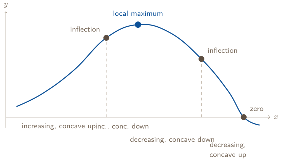
The sentence for the first stretch, in the CED’s form: on the interval from to , as increases, increases at an increasing rate; the graph is concave up. Every clause is a claim about rates, and every claim can be checked from a table.
CHECK 1 — LIMIT THE INFERENCE
No. Five rising samples prove exactly one thing: those five outputs are in increasing order. They say nothing about the inputs between them, where the function is free to dip and come back — five points sit on infinitely many functions, and only some of them are increasing. What the table supports is a candidate: under a smooth model with no other information, rising samples suggest a rising function, and rising differences suggest concave up. That is a real answer and it scores, provided you say which it is. The wording is the whole difference: “the table suggests the volume increases” earns the point that “the volume increases throughout” does not, because the second one claims evidence you were never given. Say what the representation shows, then say what it suggests.
3. RATES OF CHANGE: AVERAGE, INSTANTANEOUS, AND CHANGING
The average rate of change of over is the constant rate that would produce the same change in output over that interval:
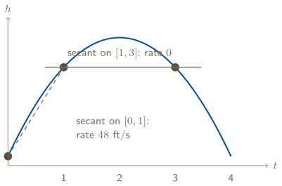
the slope of the secant through and , in output units per input unit. The rate of change at a point is how fast the output would change if the input changed there; it is approximated by average rates over small intervals containing the point, and two points’ rates are compared that way. A positive rate: the two quantities move together; negative: one rises as the other falls.
How the rate changes is the shape. Over consecutive equal-length intervals:
- a linear function has the same average rate on every interval — the rates change at a rate of zero;
- a quadratic function has average rates that form a linear pattern — the rates change at a constant rate, so the second differences are constant;
- when the rates over equal steps are increasing, the graph is concave up; decreasing, concave down.
| 0 | 1 | 2 | 3 | 4 | |
|---|---|---|---|---|---|
| 5 | 53 | 69 | 53 | 5 | |
| first differences (the rates) | 48 | 16 | |||
| second differences |
The rates fall by 32 every step: a quadratic, concave down, and the is , twice the leading coefficient. That table is the whole of Topic 1.3.
4. POLYNOMIALS AND THEIR RATES OF CHANGE: EXTREMA AND INFLECTION
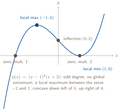
A polynomial of degree is with ; is the leading term. Where switches from increasing to decreasing it has a local maximum; from decreasing to increasing, a local minimum; a restricted domain’s included endpoint can be one too. A local extremum that beats every other output is global.
Three facts the exam tests as reasons:
- between any two distinct real zeros there is at least one local maximum or minimum — the graph has to turn to come back;
- a polynomial of even degree has a global maximum or a global minimum (both ends go the same way); a quadratic’s is its vertex;
- a point of inflection is where the rate of change switches from increasing to decreasing or back — where concavity changes.
5. ZEROS: FACTORS, MULTIPLICITY, COMPLEX PAIRS, TH DIFFERENCES, EVEN AND ODD
is a zero of when ; for a real , is a factor of if and only if is a zero. A factor repeated times gives a zero of multiplicity , and a polynomial of degree has exactly complex zeros counting multiplicity. A real zero is an -intercept and an endpoint of the intervals that solve or . A non-real zero brings its conjugate with it.
Multiplicity is the shape at the zero. Odd multiplicity: the graph crosses. Even multiplicity: the outputs keep their sign on both sides, so the graph is tangent to the axis and bounces.
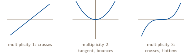
The degree from a table. Over equal-interval inputs, take successive differences of the outputs; the degree is the first for which the th differences are constant. (Card 3’s quadratic table is constant at the second round.)
Even and odd functions. An even function satisfies and is symmetric across the -axis; with even is one. An odd function satisfies and is symmetric about the origin; with odd is one. Most polynomials are neither; the test is the algebra, not the degree.
6. END BEHAVIOR OF A POLYNOMIAL: THE LEADING TERM WINS
As increases or decreases without bound, a nonconstant polynomial’s output increases or decreases without bound, and the notation is a limit: or , and the same toward . Which way is decided by the degree and the sign of the leading term, because for large the leading term dominates every lower-degree term.
| leading term | ||
|---|---|---|
| even degree, | ||
| even degree, | ||
| odd degree, | ||
| odd degree, |
Even degree: both ends the same way, like . Odd degree: opposite ways, like . The sign of flips the picture. Nothing else in the polynomial has a vote at the ends.
7. END BEHAVIOR OF A RATIONAL FUNCTION: THE QUOTIENT OF LEADING TERMS
A rational function is a quotient of two polynomials, and for large each polynomial is dominated by its leading term, so the rational function is dominated by the quotient of the leading terms. Three cases:
- the numerator dominates (higher degree): the quotient of leading terms is a nonconstant polynomial, and has that polynomial’s end behavior; if it is linear, the graph has a slant asymptote parallel to that line (division gives the line itself);
- neither dominates (equal degrees): the quotient is a constant, the horizontal asymptote ratio of leading coefficients;
- the denominator dominates: the quotient is a constant over a polynomial, and the horizontal asymptote is .
When is a horizontal asymptote the outputs get and stay arbitrarily close to as grows: , . The graph may cross a horizontal asymptote in the middle; the asymptote is a statement about the ends.
2. KEEP THE EXCLUDED INPUT
For , is a zero, a hole, or a vertical asymptote? And where is the zero?
8. ZEROS, VERTICAL ASYMPTOTES AND HOLES: THE MULTIPLICITY CONTEST
Factor the numerator and the denominator. Then, at each real zero of either:
- a zero of the numerator only, inside the domain, is a zero of — an -intercept;
- a zero of the denominator whose multiplicity there is greater than in the numerator is a vertical asymptote : the denominator is arbitrarily close to , so increases or decreases without bound, and each side gets its own limit — , ;
- a zero of the denominator whose multiplicity in the numerator is at least as large is a hole at : the factors cancel, and the hole sits at where is the value the simplified expression approaches — , the same from both sides.
The real zeros of both polynomials are the endpoints and asymptotes of the intervals that solve or : a sign chart with every one of them marked.
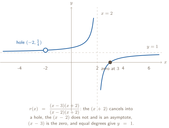
CHECK 2 — KEEP THE EXCLUDED INPUT
A hole, and the zero is at . The cancels, so for every the function equals — but cancelling is something you did to the expression, not to the function, and was never in the domain to begin with. So the graph is the line with the point lifted out of it. It is not a vertical asymptote, because nothing is left in the denominator to blow up; and it is not a zero, because a zero is a place the function takes the value , and at the function takes no value at all. The zero is where the surviving numerator vanishes: , so . The habit that protects all three answers is one line long — write the original denominator’s zeros down before you simplify anything, and carry that list to the end.
9. EQUIVALENT FORMS: WHAT EACH ONE SHOWS, DIVISION, AND THE BINOMIAL THEOREM
The factored form shows real zeros — and so -intercepts, holes, vertical asymptotes, the domain and, for a rational function, much of the range. The standard form shows the leading term, and so end behavior. Different forms of one function answer different questions, and the exam asks you to pick.
Polynomial long division writes with the remainder’s degree below the divisor’s — the same relationship as . Its use in this unit is the slant asymptote: when a rational function’s numerator is one degree above its denominator, the quotient is a line and the graph approaches it, because at the ends.
The binomial theorem expands with the th row of Pascal’s triangle as coefficients — for , the row :
so expands without multiplying it out times. Each term’s exponents sum to , and the coefficients are symmetric.
10. TRANSFORMATIONS: FOUR MOVES, APPLIED IN ORDER, TRACKED ON ONE POINT
new function | what happens to the graph | a point goes to |
|---|---|---|
| vertical translation by | |
| horizontal translation by | |
, | vertical dilation by ; reflects over the -axis | |
, | horizontal dilation by ; reflects over the -axis |
The two inside the function work backwards — moves left, compresses — because the input has to be smaller, or arrive sooner, to produce the same output. The set of points before the transformation is the preimage, after it the image, and combined transformations apply in order: dilate, then translate, unless the parentheses say otherwise. The domain and range of the image can differ from the parent’s — has domain and range , neither of which is ’s.
3. CHOOSE DEGREE FROM DIMENSIONS
A cylinder has a fixed circular base and a variable height . Is its volume a cubic function of , because volume is three-dimensional?
11. CHOOSING A MODEL, AND SAYING WHAT IT ASSUMES
The function type is read from the rates in the data or the scenario, and from its geometry:
the data or context shows | the model |
|---|---|
a roughly constant rate of change | linear |
rates that change at a roughly constant rate; or symmetric data with one maximum or minimum | quadratic |
a product of two lengths, each linear in the modeled input | quadratic if both slopes are nonzero |
a product of three lengths, each linear in the modeled input | cubic if all three slopes are nonzero |
several real zeros or several maxima and minima | a polynomial |
roughly constant nonzero th differences at equally spaced inputs | a degree- polynomial is a candidate |
points with distinct inputs | a polynomial of degree at most fits them exactly |
different behavior over different intervals | a piecewise-defined function |
two quantities inversely proportional (force and distance squared) | a rational function |
Assumptions and restrictions are part of the model, and the exam asks for them: what the model assumes stays constant; how it assumes the quantities change together; a domain restriction from the mathematics or the context (a length cannot be negative; a sheet 20 cm wide allows corner squares under 10 cm); a range restriction such as rounding to whole units. A model with its restrictions unstated is incomplete.
CHECK 3 — CHOOSE DEGREE FROM DIMENSIONS
No — , and with the base area fixed that is linear in . The word “volume” is about the units of the output; the degree is about how many of the dimensions actually move with the input, and here only one does. Cut the base variable instead — a cube of side — and is cubic, because all three dimensions are the same moving quantity. The general rule is worth writing on the page every time: a product of lengths, each of them linear in the input with a nonzero slope, is degree ; count the moving factors, not the dimensions of the answer. The same trap runs the other way with area: a rectangle of fixed width and variable length has linear area. Problem 8’s open box is the honest version — two dimensions move against one another, and the degree is what the algebra says, not what the geometry is called.
12. BUILDING THE MODEL AND USING IT, WITH UNITS
Three ways to build one. From restrictions: zeros give factors, one more point fixes the leading coefficient — with gives . From a parent: a transformation of , or moved and scaled to the scenario. From data: a linear, quadratic, cubic or quartic regression on the calculator, chosen by the pattern of the rates, reported with its coefficients to three decimal places. A piecewise model combines techniques over intervals; a rational model fits inverse proportion, , with fixed by one observation.
Applying it means answering the question that was asked: a predicted value, a rate of change, an average rate over an interval, a change in the rate — each with units extracted from the context (cubic centimeters, lumens, feet per second) and each read against the domain restriction. A prediction outside the domain is not a prediction the model makes.
PROBLEM 1
Change in tandem: the sentence, the average rate, and the rate at a point
A pool is being filled. The table gives the volume of water , in cubic meters, at time , in minutes.
| (minutes) | 0 | 1 | 2 | 3 | 4 | 5 | 6 |
|---|---|---|---|---|---|---|---|
| (cubic meters) | 0 | 0.3 | 0.8 | 1.3 | 1.7 | 2.0 | 2.2 |
(a) Describe, in the CED’s form, how changes as increases from 0 to 6, including concavity, with the evidence from the table. (b) Calculate the average rate of change of over the interval from to , with units, and say what it means. (c) Approximate the rate of change of at and at , and compare them. (d) State the domain and range of as the table gives it, and name one zero.
BEFORE YOU COMPUTE
Rung 1 and rung 2: the question is about how two quantities change together, so the answer is card 2’s sentence, and every clause in it is a claim about rates that the table can check. Before (a), compute the differences between consecutive volumes; the direction is their sign, the concavity is whether they grow or shrink. Before (c), remember that the rate at a point is not in the table — it is approximated by average rates over the smallest intervals around it, and the word “approximately” is part of the answer.
WORKING
(a) The consecutive differences, in cubic meters per minute:
All sampled volumes increase. The average rates rise (), hold, then fall (). The table suggests increasing volume across the interval, with a rate that initially rises and later falls. Under a smooth model, this suggests initial concavity up followed by concavity down. The equal middle rates do not locate an exact change of concavity, and finite samples cannot establish behavior at every intervening time.
(b) The secant slope, with the function, the interval and the units in the sentence:
Over the interval from to minutes, the volume of water increased at an average rate of cubic meters per minute — a constant rate that would have produced the same cubic meters in the same three minutes.
(c) At , the smallest intervals around it are and , with average rates and ; the rate at is approximately their middle, about cubic meters per minute. At , the intervals and give and : about . The pool is filling faster at than at , by roughly cubic meters per minute — which is what “increasing at a decreasing rate” looked like in (a).
(d) For the table as given, the domain is
and the range is
A continuous model would have additional input and output values; the table alone does not specify them. , so is a zero — the moment the pool was empty.
ANSWER
(a) sampled outputs increase; the rates suggest initial concavity up followed by concavity down under a smooth model, without establishing every intervening value (b) cubic meters per minute over (c) about at , about at : faster at (d) domain minutes; range cubic meters; zero at
WATCH OUT
Concavity from the height. The volume is rising the whole time, and a student who reads “rising” as “concave up” loses (a); concavity is about whether the rate is rising, and after it is falling while the volume still climbs. Second, a rate with no interval — “the rate is 0.4” — or no units; the CED’s own sentence carries both, and the grader looks for both. Third, in (c): reporting or as the rate at . Neither interval contains only ; the honest answer is an approximation from both sides, said as one.
CONNECTION
The differences in (a) are Unit 1’s whole method for shape: card 3 turns them into the test for linear against quadratic, card 5 into the test for degree, and card 11 into the choice of a model. And (c) is the idea AP Calculus is built on — a rate at an instant approximated by average rates over shrinking intervals — met here a year early, in a table, with the word “approximately” doing the limit’s job.
ABOUT THIS EXCERPT
This is the opening of a 36-page guide: the diagnostic tree, the full Master Toolbox, and the first worked problem. 8 more problems follow in the complete guide, each worked the same way — what to notice before you start, every step shown, and the mistake that problem invites. The complete guide is shared with families during the fit conversation.
Engineering Confidence — engineeringconfidence.one
Source and review notes
What this resource is
Complete browser edition of the public excerpt from an original Engineering Confidence AP Precalculus unit-reference packet. Every function, table and scenario was written for this guide.
- Published
- Last reviewed
- Printable edition
- 17 pages
Course reference: official College Board course page.
Read this public excerpt above, or save the PDF for printing and offline reading.
Download the 17-page PDF excerpt